English

• The urgent demand for green and renewable energy has intensified research efforts into the efficient utilization and conversion of carbon dioxide (CO₂), a central challenge in addressing both environmental and energy crisis [1–3]. The Sabatier reaction, which converts CO₂ and hydrogen (H₂) into methane (CH₄), offers a promising strategy for CO₂ valorization but conventionally requires severe operating conditions, temperatures of 300–500 ℃ and pressures of 5–30 bar [4,5]. These stringent conditions result in substantial energy consumption and pose risks such as catalyst sintering and carbon deposition [6]. Photothermal catalytic CO₂ methanation has emerged as an attractive alternative. In contrast to traditional thermocatalysis, photothermal catalysis employs solar energy through a synergistic photonic–thermal mechanism, enabling efficient CO₂ conversion under much milder conditions (120–300 ℃, atmospheric pressure). This results in reduced energy input, lower operational risks, and potentially extended catalyst lifetimes [7–9]. The combined influence of photonic and thermal energy not only facilitates reactant activation at lower temperatures but also enhances selectivity and control over the reaction environment—benefits difficult to achieve with thermocatalysis alone [10,11].

  Despite these advantages, the practical application of photothermal methanation remains limited by suboptimal methane yields, primarily due to the complexities of multi-physical field coupling [12–14]. The interactions among light absorption, heat transfer, and catalytic active sites introduce significant nonlinear threshold effects in critical parameters such as metal loading, pore size, and light intensity [15–18]. These intricate relationships are challenging to deconvolute and optimize using conventional trial-and-error methods, thereby hindering the rational design of more efficient catalytic systems [19,20]. Current research faces dual challenges of elucidating mechanistic pathways and optimizing process parameters for photothermal catalysis. On one hand, the reaction depends on intricate interdependencies among light intensity, reaction temperature, and catalyst properties (e.g., bandgap and porosity), necessitating a clear understanding of each parameter's mechanistic role to achieve effective process optimization [21]. On the other hand, most existing studies predominantly investigate single-variable effects, lacking systematic exploration of cooperative and often nonlinear synergies among multiple factors [22–25]. In particular, nonlinear threshold phenomena—such as critical behaviors in temperature, pore size, metal loading, and light intensity—must be more thoroughly understood to fully leverage photothermal technology.

  The integration of machine learning (ML), experimental data, and density functional theory (DFT) has revolutionized catalyst discovery and optimization, enabling rapid identification of key parameters and facilitating high-throughput screening [26,27]. This approach has yielded significant advances in catalyst screening for CO₂ reduction strategies, including electrocatalysis, thermocatalysis, and photocatalysis [28–31]. However, the application of these methodologies to the more complex photothermal reduction of CO₂ remains underexplored. This disparity primarily originates from the intricate multi-physical coupling inherent to photothermal catalytic systems, which produces highly nonlinear and multiscale interaction networks. The complexity of these relationships continues to obscure a comprehensive understanding of the field and constrains further development [31,32]. Therefore, the development of interpretable ML frameworks is imperative for addressing these challenges.

  To address these issues, this study proposes a transparent machine learning framework that systematically integrates experimental literature data and interpretable modeling to predict and optimize methane production in photothermal CO₂ methanation. By curating a comprehensive multi-parameter dataset and rigorously comparing advanced regression models, we identify the most effective approach for capturing the nonlinear synergies inherent in these catalytic systems. Employing SHAP and partial dependence analyses, our methodology not only provides data-driven insights into pivotal mechanistic factors but also establishes a practical tool for guiding the rational design and experimental validation of high-performance photothermal catalysts.

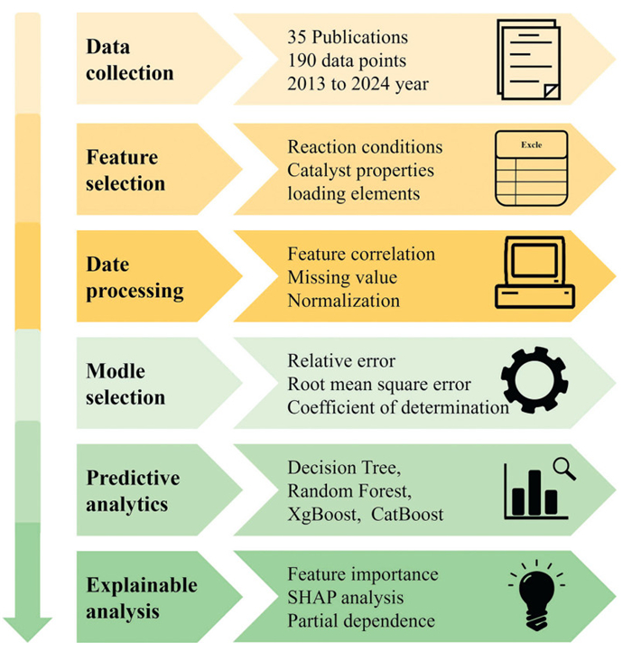
  In the data collection process, we conducted a comprehensive review of literature on CO₂ photothermal reduction from 2013.01 to 2024.08 through Web of Science using the search keyword "Photothermal catalysis and Carbon dioxide reduction". An initial literature search yielded 299 results, from which 113 relevant studies on photothermal carbon dioxide methanation were identified after screening. Further refinement based on specific data requirements, such as the presence of reaction temperature, light intensity, reaction ratios, and methane production rates, led to the selection of 35 high-quality papers. These 35 papers provided 190 high-quality data points for data collection and were used to establish a high-performance machine-learning model predicting methane production rate (Fig. S1 and Note S1 in Supporting information). The specific machine-learning framework flowchart is depicted in Fig. 1. The following assumptions and strategies were included in the data collection process. All screened data were initially accepted fairly without any preliminary judgment or bias on the validity of the data. For data that were not directly listed in tables or as text, necessary data were obtained from figures using the open-source Web Plot Digitizer software. For data collection in each literature, an average of 5 data points were taken to prevent excessive similar data from affecting the simulation results [33]. The data set included 190 columns of experimental data and 30 descriptors. It should be noted that the data originate from different research groups, and the reported protocols vary widely in reactor geometry, light-power calibration method, temperature measurement (infrared imaging vs. thermocouple), definition of steady state, and range of detected products—discrepancies that can bias the machine-learning simulations. The limited volume of literature data further constrains the statistical power required to uncover subtle mechanistic relationships. Establishing more standardized experimental reporting and expanding the dataset are therefore essential. The descriptors were roughly divided into three categories: Reaction conditions, catalyst properties, and metal loading elements. The reaction conditions include: Reaction temperature (℃), light intensity (kW/m²), reaction gas ratio, flow rate (mL/min), pressure (atm), reaction time (min), and catalyst mass (mg); the catalyst properties include: Pore size (nm), loading ratio (%), band gap (eV), pore volume (cm³/g), nanoparticle size (nm), specific surface area (m²/g); and the metal loading elements include: Ni, Ru, Rh, Ag, Cu, Co, Fe, La, Ce, Zr, Ti, Pd, Au, W, Mo, Ir, Pt. The data in the data set were analyzed through the maximum value, minimum value, average value, median value, 95% confidence interval-violin and plot methods to obtain Table S1 and Fig. S2 (Supporting information). Through the violin plot and the data in Table S1, it can be known the main centralized distribution situation of the data in the data set. When comparing the mean and median, if the mean exceeds the median, the data may show a right-skewed distribution. Conversely, if the mean is less than the median, it may indicate a left-skewed distribution. A small difference between them suggests no obvious data bias. Also, the 95% confidence interval, calculated from sample data in statistical inference, shows the range for population parameters like the mean or median, reflecting estimation precision. This study focuses on predicting the yield of photothermal CO₂ hydrogenation to methane through a systematic machine learning-driven modeling approach. The preprocessed dataset was randomly partitioned into 80% training and 20% testing subsets, with pairwise feature correlation analysis performed to mitigate multicollinearity (Fig. S3 in Supporting information for the correlation heatmap). Algorithm-specific preprocessing was applied: Neural networks and SVM models utilized StandardScaler standardization (μ = 0, σ = 1), while tree-based models (decision trees, random forests) were trained on raw data. Fourteen regression models—spanning linear regression, regularized linear models, tree ensembles, kernel methods, and neural networks—were evaluated using metrics including coefficient of determination (R²), root mean square error (RMSE), relative error (RE), and 5-fold cross-validation. Hyperparameter optimization was implemented to identify the optimal predictive model. Detailed descriptions of data processing and model selection are provided in Notes S2 and S3 (Supporting information).

  Figure 1

  

  Figure 1.  Flowchart illustrating the data analysis pipeline used in this study. The process consists of six sequential stages: (1) Data collection—comprising 190 data points from 35 publications spanning 2013 to 2024; (2) Feature selection—focused on reaction conditions, catalyst properties, and metal loading element; (3) Data processing—including feature correlation analysis, missing value handling, and normalization; (4) Model selection—evaluated by relative error, root mean square error, and coefficient of determination; (5) Predictive analytics—performed using Decision Tree, Random Forest, XGBoost, and CatBoost algorithms; and (6) Explainable analysis—encompassing feature importance, SHAP analysis, and partial dependence. Arrows indicate the direction of workflow progression.

  DownLoad: Full-Size Img PowerPoint

  After training, model interpretation is a key step to test whether the model prediction is consistent with the generalized experimental results. There are some reliable strategies (such as Shapley additive explanation, feature importance and partial dependence diagram) to explain black box models.

  SHapley Additive exPlanations (SHAP): Rooted in cooperative game theory, SHAP quantifies the marginal contribution of each feature to the predicted methane production rate. Compared with alternative explainers such as local interpretable model-agnostic explanations (LIME) or counterfactual explanations, SHAP delivers superior global and local interpretability through game-theoretic consistency and additive feature attribution, ensuring fairness and reliability in the quantification of each feature's contribution.

  Feature importance: Based on the relative influence of each variable on the machine-learning model, feature importance is expressed on a 0–100% scale; a higher score indicates a stronger impact on the output. Derived from tree-based models such as random forests, this metric excels in computational efficiency and ease of ranking key variables, and it outperforms permutation importance in the presence of correlated features by avoiding upward bias.

  Partial dependence plots (PDP): PDP illustrates the relationship between the target variable (methane production rate) and a selected set of input variables while marginalizing over all remaining inputs. Owing to visual constraints, the feature subset is restricted to univariate or bivariate cases. The dependence of each influential variable on methane production rate is further examined via partial dependence curves. Moreover, PDP intuitively reveals marginal effects and interactions, capturing non-linear relationships without extensive post-processing, thereby offering a more direct visualization than individual conditional expectation (ICE) plots.

  Upon collection of the dataset, we initially evaluated 14 machine learning models, including linear models (Linear Regression, Lasso, Ridge, ElasticNet), tree-based models (Decision Tree, Random Forest, XGBoost, Gradient Boosting Decision Tree (GBDT), CatBoost), kernel-based models (Kernel Ridge, Support Vector Machine (SVM)), and the neural network model MLPRegressor. After conducting a grid search, we further manually fine-tuned the hyperparameters to optimize the models. The best four models—Decision Tree, Random Forest, XGBoost, and CatBoost—along with their specific hyperparameter optimizations (Table S2 and Note S4 in Supporting information).

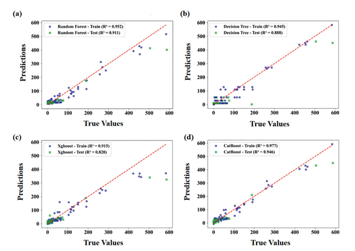
  Based on initial performance assessment using the coefficient of determination (R², Fig. S4 in Supporting information), four models—Decision Tree, Random Forest, XGBoost, and CatBoost—were identified as the top performers. Fig. 2 presents a detailed comparison of these four models by plotting their predicted versus true values for both training and test sets, with corresponding R² values. Notably, the CatBoost model achieves R² values of 0.977 on the training set and 0.946 on the test set, indicating excellent fitting accuracy. To rigorously evaluate model generalization, we further implemented K-fold cross-validation.

  Figure 2

  

  Figure 2.  Scatter plots of the coefficient of determination (R²): (a) Random Forest, (b) Decision Tree, (c) XGBoost, and (d) CatBoost models. Blue circles represent predictions for the training set and green squares represent predictions for the test set. The red dashed line indicates perfect agreement. The R² scores for both training and test datasets are shown in each panel legend.

  DownLoad: Full-Size Img PowerPoint

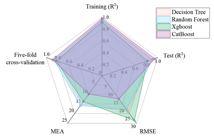
  The results, summarized in Table S2, include R², root mean square error (RMSE), mean absolute error (MAE), and cross-validation scores for each model, along with their optimized hyperparameters. CatBoost demonstrated the most robust performance, with the lowest relative RMSE (2.5%) and MAE (1.6%) across the target variable range (0–583.4 mmol g^-1 h^-1). Fig. 3 provides a visual comparison of the four models via a radar plot, incorporating metrics such as training and test R², RMSE, MAE, and five-fold cross-validation R² scores. CatBoost consistently achieved the highest values across all metrics, with an average five-fold cross-validation R² exceeding 0.88, underscoring its superior predictive capability and generalization to unseen data. Building on its demonstrated superior predictive performance, the CatBoost model was selected as the optimal approach for predicting photocatalytic hydrogenation methanation yields from carbon dioxide under varying experimental conditions. Its high accuracy enables in-depth interpretation of how different input variables affect methane production outcomes.

  Figure 3

  

  Figure 3.  Radar chart comparing the performance of four machine learning models—Decision Tree, Random Forest, XGBoost, and CatBoost—across five evaluation metrics: Training R², Test R², five-fold cross-validation R², root mean square error (RMSE), and mean absolute error (MEA). The R² axes range from 0 to 1 (higher values indicate better performance), while RMSE and MEA axes range from 0 to 30/25 (lower values indicate better performance).

  DownLoad: Full-Size Img PowerPoint

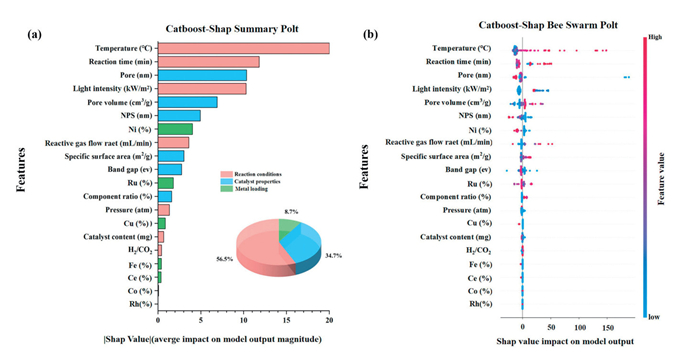
  To elucidate the determinants driving model predictions, SHAP analyses were conducted to assess feature importance and the directionality of each variable's impact. Fig. 4a presents a SHAP summary plot, where features are ranked by their average impact on the model's output. The analysis identifies temperature, pore size, and gas flow rate as the three most influential factors in predicting methane yield. The accompanying pie chart categorizes input features by type, revealing that reaction conditions account for the largest proportion of model influence (56.5%), followed by catalyst properties (34.7%) and metal loading (8.7%).

  Figure 4

  

  Figure 4.  SHAP analysis of feature importance for the CatBoost model. (a) SHAP summary plot ranking features by their average impact on model output, with a pie chart illustrating the relative contributions from catalyst properties, reaction conditions, and loading with metals. (b) SHAP bee swarm plot visualizing the effect of each feature value on model predictions, where features are listed vertically and each point's color indicates the relative feature value (blue: low, pink: high).

  DownLoad: Full-Size Img PowerPoint

  Fig. 4b displays a SHAP bee swarm plot, where each point represents an individual prediction, colored by the magnitude of the underlying feature value (from low, blue, to high, pink). This visualization reveals not only the importance of each variable but also how high or low values influence the prediction. For example, the SHAP values of temperature are mostly positive, and they increase with rising temperature (color shifts from blue to red), showing that high temperatures significantly boost methane production. Conversely, the SHAP values of pore size are largely negative, decreasing as pore size increases (color also shifts from blue to red), which indicates that larger pores have a clearly negative impact on methane production.

  While Fig. 4 focuses on SHAP-based interpretability, further quantitative analysis of single feature effects can be performed through univariate PDPs, which illustrate the nonlinear relationships between individual features and the target variable—these are discussed separately for additional mechanistic insight.

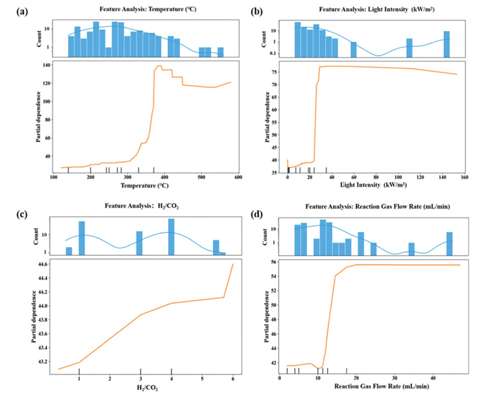
  Fig. 5 presents the PDPs for four key reaction conditions: Temperature, light intensity, H₂/CO₂ ratio, and gas flow rate. Each subplot displays the marginal effect of a single feature on the predicted methane production rate, with the accompanying histogram indicating the experimental frequency for each parameter. The mathematical definition of PDPs and the rationale for using them instead of Accumulated Local Effects (ALEs) are provided in Note S5 (Supporting information).

  Figure 5

  

  Figure 5.  Feature analysis for four reaction conditions: (a) Temperature (℃), (b) light intensity (kW/m²), (c) H₂/CO₂ ratio, and (d) gas flow rate (mL/min). Each panel displays the distribution of feature values in the dataset (upper histogram) alongside the corresponding partial dependence plot (lower curve).

  DownLoad: Full-Size Img PowerPoint

  According to Fig. 5a, the methane production rate remains relatively stable between 100 ℃ and 300 ℃, but increases sharply as temperature rises beyond 300 ℃. After 400 ℃, the rate plateaus, indicating diminishing returns at higher temperatures. This threshold effect is widely observed in experiments: Experimental evidence has shown that increasing the reaction temperature from 282 ℃ to 383 ℃ with Co-PS@SiO₂ can lead to a tenfold increase in methane production rate [34]. Similarly, other catalysts, such as Ag₂₄Au/meso‑Co₃O₄ [35], Ni-based, and Ru-based catalysts [36,37], display substantial yield increases when passing from 300 ℃ to 400 ℃, suggesting a critical temperature range where catalytic activity is significantly enhanced. At lower temperatures (< 200 ℃), the high CO₂ bond energy (~806 kJ/mol) limits dissociation, favoring the RWGS reaction as the rate-limiting step due to its lower activation barrier, leading to CO dominance [38,39]. In the optimal 250–370 ℃ range, photothermal synergies enhance energy transfer via localized heating and photogenerated carriers, activating CO₂ more efficiently and shifting the rate-limiting step toward intermediate hydrogenation, which boosts methane yield with minimal carbon deposition [40]. Above 400 ℃, the exothermic methanation equilibrium reverses, exacerbating RWGS competition and carbon buildup, reducing selectivity.

  Regarding illumination intensity (Fig. 5b), methane production rises steeply up to 30–40 kW/m² before plateauing or slightly declining. At lower intensities, increased illumination boosts catalyst surface temperature via photothermal heating and enhances localized surface plasmon resonance (LSPR) in metal nanoparticles, facilitating CO₂ activation and hydrogenation [40–43]. This promotes charge carrier generation and intermediate migration to active sites, improving yield and selectivity. At higher intensities, potential nonuniform heating or intermediate buildup (e.g., CO accumulation) may reduce selectivity, as supported by experimental reports of similar trends [44,45].

  As observed in Figs. 5a and b, the dependence on light intensity exhibits a superlinear trend, which, according to prior reports [46], indicates a mechanism primarily driven by thermal effects rather than a linear photochemical-dominated process. Given that both photochemical and thermal mechanisms may coexist in photothermal CO₂ hydrogenation, we note that the observed superlinearity points to thermal effects as the dominant pathway in our system, with potential minor photochemical influences at lower intensities.

  The PDP in Fig. 5c indicates that methane production rate increases significantly when the H₂/CO₂ ratio exceeds 4.0, with an optimal range between 4.0 and 6.0. Mechanistically, a higher H₂/CO₂ ratio enhances the deep hydrogenation of CO₂ to CH₄ by providing abundant hydrogen for the sequential reduction steps (CO₂ → CO → CH₄), which suppresses the competing reverse water-gas shift (RWGS) reaction that favors CO formation [47–49]. This shift improves methane selectivity by accelerating the conversion of CO intermediates at active sites and optimizes thermodynamic equilibrium, reducing carbon deposition risks that could deactivate the catalyst. These effects align with experimental observations where elevated reductant ratios lead to higher CO₂ conversion and methane yields, as the excess H₂ mitigates kinetic limitations in hydrogenation [49].

  This aligns with previous findings that demonstrate enhanced CO₂ conversion to methane at higher reductant ratios. As shown in Fig. 5d, methane production initially rises with increasing gas flow rate, plateauing around 30 mL/min. From a fundamental perspective, moderate increases in flow rate enhance mass transfer by improving reactant diffusion to the catalyst surface, ensuring more efficient contact and higher conversion rates. However, at higher flow rates, the reduced residence time limits the opportunity for complete hydrogenation of intermediates, leading to incomplete conversion of CO to CH₄ and thus lower selectivity. This threshold behavior is consistent with prior studies on flow dynamics in fixed-bed reactors, where excessive flow can introduce transport limitations without benefiting overall performance [49].

  Overall, the PDPs provide valuable quantitative insight into the nonlinear and threshold-dependent impacts of key operational parameters, while the data distribution histograms highlight the experimental coverage and reliability of these model-derived trends.

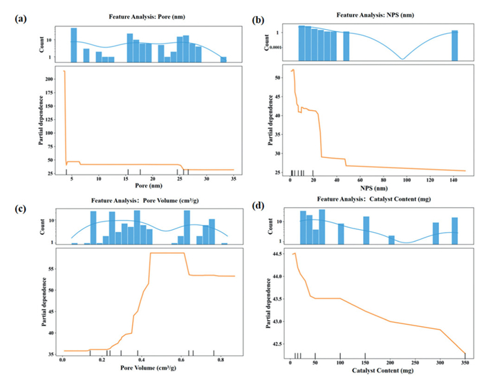
  Fig. 6 presents PDPs for key catalyst characteristics: Pore size, nanoparticle size, pore volume, and catalyst content. As shown in Fig. 6a, methane production rate decreases sharply as pore size increases, with the highest rates observed at pore sizes below 4 nm. However, the rapid decline beyond this point may be influenced by limited data in the larger pore range, as indicated by the histogram. Mechanistically, smaller pore sizes restrict the growth of metal nanoparticles, ensuring better dispersion and minimizing aggregation [50,51]. This leads to smaller, more uniform nanoparticles that promote higher surface area, improved light absorption, and greater catalytic activity [51,52]. Fig. 6b demonstrates a similar inverse trend: Smaller nanoparticles are associated with higher methane yields. This can be attributed to enhanced surface area, better heat transfer, and more available active sites, which collectively boost photothermal efficiency and catalytic performance [53–55]. According to Fig. 6c, methane production rate initially increases with pore volume, reaching an optimum between approximately 0.45 and 0.65 cm³/g [56,57]. This result aligns well with literature indicating that optimal pore volume enhances CO₂ adsorption capacity in porous materials, an essential factor for effective catalysis. Fig. 6d reveals a pronounced maximum in methane production at a catalyst content of around 10 mg. Below this value, thinner catalyst layers facilitate greater light penetration and a stronger photothermal effect. Additionally, lower catalyst mass reduces heat capacity and heat accumulation, improving the conversion efficiency. At higher loadings, however, the catalytic layer becomes thicker, which restricts light penetration, potentially increases heat capacity, and can reduce overall photothermal efficiency [58]. In addition to the effects of catalyst content on light penetration and heat capacity (Fig. 6d), radiative heat loss must also be considered, particularly at elevated temperatures where it follows the Stefan-Boltzmann law (proportional to T^⁴). High-emissivity catalysts can exacerbate this loss, potentially reducing local temperatures and catalytic efficiency. Strategies to mitigate this, such as engineering low-emissivity surfaces or optimizing reactor insulation, could enhance photothermal performance, as demonstrated in recent studies [59]. Future work incorporating emissivity measurements would further refine these insights.

  Figure 6

  

  Figure 6.  Feature analysis plots for four catalyst characteristics: (a) Pore (nm), (b) NPS (nm), (c) pore volume (cm³/g), and (d) catalyst content (mg). Each panel displays the distribution of feature values in the dataset (upper histogram) alongside the corresponding partial dependence plot (lower curve).

  DownLoad: Full-Size Img PowerPoint

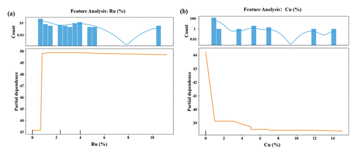
  Figs. 7a and b illustrate the impact of different metal loading (%) on the methane production rate. Fig. 7a reveals that the methane production rate initially rises with increasing Ru loading, peaks within the 1.5%−3% range, and subsequently declines when the loading exceeds 3%. This decline is attributed to excessive Ru loading (%) causing particle agglomeration, reducing active sites, and disrupting metal-support interactions [40]. Concurrently, research has established that within the 1%−5% loading range, the 3% Ru/CeO₂ catalyst exhibits optimal Ru reduction, strong metal-support interaction, and high CO₂ adsorption and hydrogenation capabilities, aligning with our predictions [60]. Fig. 7b indicates that higher Cu loading (%) lower the methane production rate. This is because Cu's electronic properties lower the Gibbs free energy barrier for CO generation, enhancing CO selectivity and reducing methane selectivity in the reaction induced by nonthermal effects over CuNi/CeO₂ [24,61]. Additional univariate partial dependence plots of how pressure, band gap, specific surface area, and Fe percentage affect methane yield in photothermal CO₂ hydrogenation showed in Fig. S5 (Supporting information). The results reveal that methane yield peaks at moderate pressure and specific surface area, is strongly enhanced by narrow band gaps (though wide band gaps can also offer redox benefits), and decreases with higher Fe percentage due to occupation of oxygen vacancies and fewer active sites. Based on our dataset and PDP, Ru shows a parabolic trend in methane yield with loading, increasing initially due to enhanced H₂ activation and photothermal heat generation, then decreasing likely from site blocking or aggregation; this results in higher overall rates owing to its strong CO₂ dissociation and dual reaction pathways (HCOO and CO) [62–64]. Cu exhibits a monotonic decrease in yield with increasing loading, attributed to its moderate activity and sensitivity to oxygen defects, leading to lower rates unless optimized for cooperative effects, primarily via CO-dominated pathways with limited H supply [61,63]. Fe demonstrates robust but variable performance, with yields influenced by its role in C—O bond breaking, though often constrained by side reactions favoring CO or C_2⁺ products, resulting in rates that are generally lower than Ru in photothermal contexts due to its propensity for C—C coupling [9,63].

  Figure 7

  

  Figure 7.  Feature analysis plots for loaded metals: (a) Ru (%), (b) Cu (%). Each panel displays the distribution of feature values in the dataset (upper histogram) alongside the corresponding partial dependence plot (lower curve).

  DownLoad: Full-Size Img PowerPoint

  Overall, these analyses highlight how mesoscale and microscale catalyst features, such as pore structure and particle size, interact to influence methane production. It is also important to consider the data distribution, as the reliability of PDP trends depends on experimental coverage in each feature's range. Although ALE plots are computationally faster and avoid bias from correlated features, we chose PDP for bivariate analysis because PDPs provide a more intuitive and direct visualization of complex feature interactions. By presenting the average predicted outcome across all combinations of two features, PDPs clearly show the joint effects of feature pairs on methane production without requiring complicated second-order calculations. Moreover, PDPs are easier to interpret, with axes that explicitly display how variations in feature values relate to changes in the predicted response.

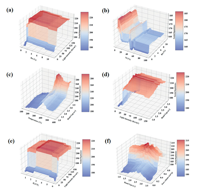
  Unraveling the mechanisms of photothermal catalytic CO₂ methanation is challenging due to complex, nonlinear interactions among reaction conditions, catalyst properties, and metal loading characteristics—factors not easily isolated by conventional methods. Traditional single-variable approaches often fail to capture these real-world synergies. By leveraging advanced machine learning models and bivariate PDP analyses, it is now feasible to quantitatively assess synergistic effects between interacting parameters, enabling a more holistic interpretation of photothermal catalysis. Fig. 8 presents bivariate PDPs for parameter pairs, selected based on established experimental findings and mechanistic reasoning.

  Figure 8

  

  Figure 8.  Bivariate partial dependence surface plots showing interactions between key parameters for methane production rate. Plots illustrate the joint effects of: (a) Ru (%) and light intensity (kW/m²); (b) Ru (%) and Ni (%); (c) temperature (℃) and band gap (eV); (d) light intensity (kW/m²) and band gap (eV); (e) H₂/CO₂ ratio and light intensity (kW/m²); and (f) band gap (eV) and pore volume (cm³/g). Color gradients represent the predicted methane production rate, capturing synergistic effects between each feature pair.

  DownLoad: Full-Size Img PowerPoint

  By jointly analyzing the relationship between ruthenium content and light intensity, it can be found that they exhibit a synergistic effect. When the ruthenium loading is maintained at a moderate level (< 4%) and the light intensity is low (< 30 kW/m²), Ru, due to its uniform dispersion, can form a strong metal-support interaction (SMSI), promoting the transfer of photo-induced electrons from the support to Ru. This effectively enhances charge separation and oxygen vacancy formation, thereby improving methane yield. However, when the ruthenium content exceeds 4% or the light intensity exceeds 30 kW/m², excessive loading causes nanoparticle aggregation, reducing active sites. Moreover, under high light intensity, a thermal gradient can be generated, inducing local sintering of the support. Ultimately, this diminishes the reaction activity and selectivity [65–67].

  Thus, balanced co-catalyst loading and photothermal input are key for optimal conversion. Ni/Ru ratios and Ru levels (Fig. 8b) determine alloy characteristics, electron transfer, and surface structure. Bimetallic Ni-Ru catalysts lower activation barriers and bandgaps, as shown by DFT calculations, and improve dispersion per BET experiments. However, only an optimal Ni: Ru ratio maximizes these synergistic benefits, as excessive Ru reduces performance [38]. Bandgap paired with temperature (Fig. 8c) reveals that wide-bandgap materials (> 3.1 eV) benefit most from elevated temperatures due to enhanced UV absorption, improved redox potential, and thermally-induced oxygen vacancies, all supporting deep CO₂ reduction [39,68,69]. With light intensity (Fig. 8d), narrow bandgaps (2.0–2.5 eV) and moderate illumination (35–40 kW/m²) extend visible absorption and carrier lifetimes. Too much light, however, destabilizes intermediates and shifts selectivity [24,70]. The interplay of H₂/CO₂ ratio and light intensity (Fig. 8e) yields a volcano-shaped curve with optimal methane production at a 4:1 ratio and 25–30 kW/m². Excessive H₂ causes competitive adsorption, reducing active sites, while high light intensities generate intermediates that cannot be efficiently converted if hydrogen is too abundant, leading to diminished yields [45,71]. Bandgap and pore volume (Fig. 8f) together optimize light absorption and substrate diffusion. Maximum methane yield occurs for bandgaps of 1.5–2.5 eV and pore volumes of 0.4–0.6 cm³/g, due to enhanced visible absorption, efficient light trapping, uniform heat distribution, and improved metal dispersion [72].

  Additional bivariate partial dependence plots of how H₂/CO₂ ratio, gas flow rate, pore volume, nanoparticle size, band gap, and pressure interact to affect methane yield in photothermal CO₂ hydrogenation are presented in Fig. S6 (Supporting information). The results reveal that optimal combinations, such as balanced H₂/CO₂ ratio with gas flow rate, appropriate pore volume with gas flow rate, smaller nanoparticle size with narrow band gap, and moderate H₂/CO₂ ratio with pressure—synergistically maximize methane yield by enhancing mass transfer, catalyst utilization, light absorption, and suppressing side reactions.

  While traditional univariate analysis provides valuable insight into the individual effects of key parameters, such as temperature, light intensity, or metal loading, on photothermal CO₂ methanation, it inherently overlooks the intricate interactions and nonlinearities that govern real-world catalytic performance. In contrast, bivariate analysis, as demonstrated by our machine-learning-driven partial dependence exploration, enables quantitative assessment of synergistic effects between parameter pairs. This approach uncovers cooperation between variables, such as Ru content and light intensity, Ni/Ru ratio, or bandgap and pore volume, that not only shapes activity thresholds but also reveals optimal regimes inaccessible to simple one-factor studies. Notably, bivariate analysis clarifies the trade-offs and coordination required among operational and material features to maximize methane yield and selectivity, providing a more holistic and mechanistic understanding of catalyst function. Crucially, the integration of advanced machine learning models, especially those with high interpretability such as CatBoost coupled with SHAP and PDP analyses, empowers researchers to dissect complex, high-dimensional data and to identify hidden, often nonlinear cooperative effects that classical experimentation cannot reliably resolve. This data-driven strategy greatly enhances both mechanistic comprehension and practical optimization, charting a pathway for the rational design of next-generation photothermal catalysts. As this work illustrates, machine learning is not solely a tool for prediction, but a powerful engine for discovering, quantifying, and exploiting synergistic phenomena in advanced catalytic systems.

  In summary, this work demonstrates that interpretable machine learning, underpinned by comprehensive literature-derived datasets, offers powerful capabilities for unraveling and optimizing the multifaceted parameter space of photothermal CO₂ methanation. The CatBoost model, selected for its superior predictive accuracy and transparency, enabled detailed mechanistic dissection of the interdependencies among reaction conditions, catalyst features, and metal loading elements. Both univariate and bivariate analyses revealed key nonlinear and synergistic effects, particularly involving temperature, pore size, gas flow rate, and Ru loading, that govern methane output. Beyond predictive accuracy, the integration of SHAP and PDP tools provides actionable insights for catalyst development and process optimization, moving the field beyond conventional trial-and-error. These findings underline the transformative potential of machine learning in advancing carbon-neutral energy strategies, setting a foundation for the rational, data-driven design of next-generation photothermal catalytic systems.

  CRediT authorship contribution statement

  Zeai Huang: Conceptualization. Rui Deng: Writing – original draft, Visualization, Data curation. Ruiyang Zhang: Methodology. Renze Li: Methodology. Sinan Liu: Methodology. Jundao Wu: Visualization. Rustem Zairov: Visualization. Oleg G. Sinyashin: Visualization. Ying Zhou: Conceptualization.

  Declaration of competing interest

  The authors declare no competing financial interest.

  Acknowledgments

  This work was supported by the National Science Fund for Distinguished Young Scholars of China (No. 52325401), the National Natural Science Foundation of China for Youths (Nos. W2412080, 22209136), and RSF (No. 25-43-00131).

  Supplementary materials

  Supplementary material associated with this article can be found, in the online version, at doi:10.1016/j.cclet.2025.111909.

  
  
• 1. [1]

     X. He, S. Liang, N. Li, et al., J. Alloys Compd. 994 (2024) 174698. doi: 10.1016/j.jallcom.2024.174698

  2. [2]

     Z. Li, R. Shi, J. Zhao, et al., Nano Res. 14 (2021) 4828–4832. doi: 10.1007/s12274-021-3436-6

  3. [3]

     Q. Li, Y. Gao, M. Zhang, et al., Appl. Catal. B 303 (2022) 120905. doi: 10.1016/j.apcatb.2021.120905

  4. [4]

     M. Younas, L.L. Kong, M.J.K. Bashir, et al., Energ. Fuel. 30 (2016) 8815–8831. doi: 10.1021/acs.energyfuels.6b01723

  5. [5]

     M.A.A. Aziz, A.A. Jalil, S. Triwahyono, et al., Green Chem. 17 (2015) 2647–2663. doi: 10.1039/C5GC00119F

  6. [6]

     Y. Cui, S. He, J. Yang, et al., Molecules 29 (2024) 374. doi: 10.3390/molecules29020374

  7. [7]

     V. Golovanova, M.C. Spadaro, J. Arbiol, V. Golovanov, et al., Appl. Catal. B 291 (2021) 120038. doi: 10.1016/j.apcatb.2021.120038

  8. [8]

     Y. Li, J. Hao, H. Song, et al., Nat. Commun. 10 (2019) 2359. doi: 10.1038/s41467-019-10304-y

  9. [9]

     G. Chen, R. Gao, Y. Zhao, et al., Adv. Mater. 30 (2018) 1704663. doi: 10.1002/adma.201704663

  10. [10]

      S. Yunes, U.P. Kim, H. Nguyen, et al., Chemistry 3 (2021) 1157–1165. doi: 10.3390/chemistry3040084

  11. [11]

      M. Tommasi, S.N. Degerli, G. Ramis, et al., Chem. Eng. Res. 201 (2024) 457–482 Des.

  12. [12]

      C. Sang Hun, S. Inhak, D. Wan Jae, Energy Mater. 5 (2025) 500062.

  13. [13]

      A. Beniwal, A. Bagaria, T.Y. Chen, et al., Sustain. Energy Fuels 9 (2025) 2261–2286. doi: 10.1039/d5se00167f

  14. [14]

      C. Molinet-Chinaglia, S. Shafiq, P. Serp, ChemCatChem 16 (2024) e202401213. doi: 10.1002/cctc.202401213

  15. [15]

      B. Guene Lougou, B.X. Geng, R.M. Pan, et al., Rare Met. 43 (2024) 2913–2939. doi: 10.1007/s12598-024-02638-4

  16. [16]

      X. Lin, S. Wang, W. Tu, et al., Catal. Sci. Technol. 9 (2019) 731–738. doi: 10.1039/c8cy02329h

  17. [17]

      Y. Zhou, P. Zheng, J. Gao, et al., ACS Catal. 14 (2024) 14285–14296. doi: 10.1021/acscatal.4c02149

  18. [18]

      Y. Wang, Y. Liu, L. Tan, et al., J. Mater. Chem. A 11 (2023) 26804–26811. doi: 10.1039/d3ta05938c

  19. [19]

      H. Liu, L. Shi, Q. Zhang, et al., Chem. Commun. 57 (2021) 1279–1294. doi: 10.1039/d0cc07144g

  20. [20]

      D. Mateo, J.L. Cerrillo, S. Durini, et al., Chem. Soc. Rev. 50 (2021) 2173–2210. doi: 10.1039/d0cs00357c

  21. [21]

      J. Zhang, H. Chen, X. Duan, et al., Mater. Today 68 (2023) 234–253. doi: 10.3390/bios13020234

  22. [22]

      S. Khan, X. Dai, T. Ali, et al., Int. J. Hydrog. Energy 48 (2023) 24756–24787. doi: 10.1016/j.ijhydene.2022.09.224

  23. [23]

      H. Ge, Y. Kuwahara, K. Kusu, et al., Appl. Catal. B 317 (2022) 121734. doi: 10.1016/j.apcatb.2022.121734

  24. [24]

      X. Yue, K. Wang, Z. Yang, et al., Chem. Eng. J. 458 (2023) 141491. doi: 10.1016/j.cej.2023.141491

  25. [25]

      F.F.Y. Wan, R.X. Sun, J. Zhang, et al., Acta Phys. Chim. Sin. 39 (2023) 2212042. doi: 10.3866/pku.whxb202212042

  26. [26]

      M. Tamtaji, H. Gao, M.D. Hossain, et al., J. Mater. Chem. A 10 (2022) 15309–15331. doi: 10.1039/d2ta02039d

  27. [27]

      L.E.B. Lucchetti, J.M. de Almeida, S. Siahrostami, EES Catal. 2 (2024) 1037–1058. doi: 10.1039/d4ey00104d

  28. [28]

      Z. Gariepy, G. Chen, A. Xu, et al., Energy Adv. 2 (2023) 410–419. doi: 10.1039/d2ya00316c

  29. [29]

      M. Suvarna, T.P. Araújo, J. Pérez-Ramírez, Appl. Catal. B 315 (2022) 121530. doi: 10.1016/j.apcatb.2022.121530

  30. [30]

      D. Saadetnejad, B. Oral, E. Can, et al., Int. J. Hydrog. Energy 47 (2022) 19655–19668. doi: 10.1016/j.ijhydene.2022.02.030

  31. [31]

      J. Zhang, C. Wang, S. Huang, et al., Joule 7 (2023) 1832–1851. doi: 10.1016/j.joule.2023.06.003

  32. [32]

      M. Steiner, M. Reiher, Top. Catal. 65 (2022) 6–39. doi: 10.1007/s11244-021-01543-9

  33. [33]

      T. Toyao, Z. Maeno, S. Takakusagi, et al., ACS Catal. 10 (2020) 2260–2297. doi: 10.1021/acscatal.9b04186

  34. [34]

      K. Feng, S. Wang, D. Zhang, et al., Adv. Mater. 32 (2020) 2000014. doi: 10.1002/adma.202000014

  35. [35]

      Y. Xiong, X. Liu, Y. Hu, et al., Nano Res. 15 (2022) 4965–4972. doi: 10.1007/s12274-022-4133-9

  36. [36]

      Q. Li, C. Wang, H. Wang, et al., Angew. Chem. Int. Ed. 63 (2024) e202318166. doi: 10.1002/anie.202318166

  37. [37]

      H. Wang, Q. Li, J. Chen, et al., Mater. Chem. A 12 (2024) 15803–15813. doi: 10.1039/d4ta01821d

  38. [38]

      X. Ding, X. Liu, J. Cheng, et al., Fuel 357 (2024) 129779. doi: 10.1016/j.fuel.2023.129779

  39. [39]

      W.K. Fan, M. Tahir, H. Alias, ACS Appl. Mater. Interfaces 15 (2023) 54353–54372. doi: 10.1021/acsami.3c10022

  40. [40]

      C. Guo, Y. Tang, Z. Yang, et al., ACS Nano 17 (2023) 23761–23771. doi: 10.1021/acsnano.3c07630

  41. [41]

      H. Jiang, L. Wang, H. Kaneko, et al., Nat. Catal. 6 (2023) 519–530. doi: 10.1038/s41929-023-00970-z

  42. [42]

      S. Liu, X. Wang, Y. Chen, et al., Adv. Mater. 36 (2024) 2311957. doi: 10.1002/adma.202311957

  43. [43]

      H. Wang, Q. Li, J. Chen, et al., Adv. Sci. 10 (2023) 2304406. doi: 10.1002/advs.202304406

  44. [44]

      Q. Li, X. Zhu, C. Li, et al., Int. J. Hydrog. Energy 91 (2024) 488–495. doi: 10.1016/j.ijhydene.2024.10.135

  45. [45]

      X. Chen, Q. Li, M. Zhang, et al., ACS Appl. Mater. Interfaces 12 (2020) 39304–39317. doi: 10.1021/acsami.0c11576

  46. [46]

      S. Liu, Z. Wu, Z. Zhu, et al., Nat. Commun. 16 (2025) 2245. doi: 10.1038/s41467-025-57569-0

  47. [47]

      A. Swapnesh, V.C. Srivastava, I.D. Mall, Chem. Eng. Technol. 37 (2014) 1765–1777. doi: 10.1002/ceat.201400157

  48. [48]

      A. Gouda, K. Hannouche, A. Mohan, et al., Nat. Commun. 16 (2025) 695. doi: 10.1038/s41467-025-55891-1

  49. [49]

      A. Supaokit, V. Verma, W.C. Wang, et al., Appl. Catal. A 691 (2025) 120073. doi: 10.1016/j.apcata.2024.120073

  50. [50]

      L.L. Battiston, D.K.D. Oliveira, P.L.M. Lião, et al., ChemNanoMat 9 (2023) e202300264. doi: 10.1002/cnma.202300264

  51. [51]

      W. Zhang, K. Zhu, W. Ren, et al., Adv. Mater. Interfaces 9 (2022) 2101528. doi: 10.1002/admi.202101528

  52. [52]

      F. Subhan, S. Aslam, Z. Yan, et al., Micropor. Mesopor. Mater. 337 (2022) 111927. doi: 10.1016/j.micromeso.2022.111927

  53. [53]

      C. Lv, X. Bai, S. Ning, et al., ACS Nano 17 (2023) 1725–1738. doi: 10.1021/acsnano.2c09025

  54. [54]

      Y. Cui, X. Liang, J. Wang, et al., Energy Chem. 103 (2025) 888–910. doi: 10.1016/j.jechem.2024.12.045

  55. [55]

      P. Serna-Gallén, K. Mužina, Nano Mater. Sci. 8 (2026) 534–555. doi: 10.1016/j.nanoms.2024.10.009

  56. [56]

      M. Sevilla, A.B. Fuertes, Energy Environ. Sci. 4 (2011) 1765–1771. doi: 10.1039/c0ee00784f

  57. [57]

      Z. Bao, L. Yu, Q. Ren, et al., J. Colloid Interface Sci. 353 (2011) 549–556. doi: 10.1016/j.jcis.2010.09.065

  58. [58]

      Z. Yang, Z.Y. Wu, Z. Lin, et al., Nat. Commun. 15 (2024) 7599. doi: 10.1038/s41467-024-51896-4

  59. [59]

      K. Yu, K. Feng, M. Cai, et al., ACS Nano 19 (2025) 18674–18685. doi: 10.1021/acsnano.5c03061

  60. [60]

      S. López-Rodríguez, A. Davó-Quiñonero, E. Bailón-García, et al., Mol. Catal. 515 (2021) 111911.

  61. [61]

      Z. Yang, M. Zeng, K. Wang, et al., Fuel 315 (2022) 123186. doi: 10.1016/j.fuel.2022.123186

  62. [62]

      S. Cai, M. Zhang, J. Li, et al., Sol. RRL 5 (2021) 2000313. doi: 10.1002/solr.202000313

  63. [63]

      Y. Li, R. Li, Z. Li, et al., Sol. RRL 6 (2022) 2200493. doi: 10.1002/solr.202200493

  64. [64]

      Y. Bu, K. Wenderich, N.T. Costa, et al., Molecules 30 (2025) 2577. doi: 10.3390/molecules30122577

  65. [65]

      N. Kong, B. Han, Z. Li, et al., ACS Appl. Nano Mater. 3 (2020) 3028–3033. doi: 10.1021/acsanm.0c00383

  66. [66]

      D. Mateo, J. Albero, H. García, Joule 3 (2019) 1949–1962. doi: 10.1016/j.joule.2019.06.001

  67. [67]

      M. Novoa-Cid, H.G. Baldovi, Nanomaterials 10 (2020) 2212. doi: 10.3390/nano10112212

  68. [68]

      X. Ding, X. Liu, J. Cheng, et al., Catal. Sci. Technol. 12 (2022) 4740–4752. doi: 10.1039/d2cy00439a

  69. [69]

      V. Werner, F.B. Lora, Z. Chai, et al., RSC Sustain. 2 (2024) 1738–1752. doi: 10.1039/d4su00096j

  70. [70]

      T. Li, Z.Y. Zhang, D.C. Luo, et al., Nano Res. 17 (2024) 7945–7956. doi: 10.1007/s12274-024-6796-x

  71. [71]

      Y. Chen, Y. Zhang, G. Fan, et al., Joule 5 (2021) 3235–3251. doi: 10.1016/j.joule.2021.11.009

  72. [72]

      Y. Zhang, J. Shi, J. Ju, et al., Sep. Purif. Technol. 356 (2025) 129984. doi: 10.1016/j.seppur.2024.129984

• 

  Figure 1  Flowchart illustrating the data analysis pipeline used in this study. The process consists of six sequential stages: (1) Data collection—comprising 190 data points from 35 publications spanning 2013 to 2024; (2) Feature selection—focused on reaction conditions, catalyst properties, and metal loading element; (3) Data processing—including feature correlation analysis, missing value handling, and normalization; (4) Model selection—evaluated by relative error, root mean square error, and coefficient of determination; (5) Predictive analytics—performed using Decision Tree, Random Forest, XGBoost, and CatBoost algorithms; and (6) Explainable analysis—encompassing feature importance, SHAP analysis, and partial dependence. Arrows indicate the direction of workflow progression.

  下载: 全尺寸图片 幻灯片
  

  Figure 2  Scatter plots of the coefficient of determination (R²): (a) Random Forest, (b) Decision Tree, (c) XGBoost, and (d) CatBoost models. Blue circles represent predictions for the training set and green squares represent predictions for the test set. The red dashed line indicates perfect agreement. The R² scores for both training and test datasets are shown in each panel legend.

  下载: 全尺寸图片 幻灯片
  

  Figure 3  Radar chart comparing the performance of four machine learning models—Decision Tree, Random Forest, XGBoost, and CatBoost—across five evaluation metrics: Training R², Test R², five-fold cross-validation R², root mean square error (RMSE), and mean absolute error (MEA). The R² axes range from 0 to 1 (higher values indicate better performance), while RMSE and MEA axes range from 0 to 30/25 (lower values indicate better performance).

  下载: 全尺寸图片 幻灯片
  

  Figure 4  SHAP analysis of feature importance for the CatBoost model. (a) SHAP summary plot ranking features by their average impact on model output, with a pie chart illustrating the relative contributions from catalyst properties, reaction conditions, and loading with metals. (b) SHAP bee swarm plot visualizing the effect of each feature value on model predictions, where features are listed vertically and each point's color indicates the relative feature value (blue: low, pink: high).

  下载: 全尺寸图片 幻灯片
  

  Figure 5  Feature analysis for four reaction conditions: (a) Temperature (℃), (b) light intensity (kW/m²), (c) H₂/CO₂ ratio, and (d) gas flow rate (mL/min). Each panel displays the distribution of feature values in the dataset (upper histogram) alongside the corresponding partial dependence plot (lower curve).

  下载: 全尺寸图片 幻灯片
  

  Figure 6  Feature analysis plots for four catalyst characteristics: (a) Pore (nm), (b) NPS (nm), (c) pore volume (cm³/g), and (d) catalyst content (mg). Each panel displays the distribution of feature values in the dataset (upper histogram) alongside the corresponding partial dependence plot (lower curve).

  下载: 全尺寸图片 幻灯片
  

  Figure 7  Feature analysis plots for loaded metals: (a) Ru (%), (b) Cu (%). Each panel displays the distribution of feature values in the dataset (upper histogram) alongside the corresponding partial dependence plot (lower curve).

  下载: 全尺寸图片 幻灯片
  

  Figure 8  Bivariate partial dependence surface plots showing interactions between key parameters for methane production rate. Plots illustrate the joint effects of: (a) Ru (%) and light intensity (kW/m²); (b) Ru (%) and Ni (%); (c) temperature (℃) and band gap (eV); (d) light intensity (kW/m²) and band gap (eV); (e) H₂/CO₂ ratio and light intensity (kW/m²); and (f) band gap (eV) and pore volume (cm³/g). Color gradients represent the predicted methane production rate, capturing synergistic effects between each feature pair.

  下载: 全尺寸图片 幻灯片
•