Table 1.
48 Allergenic Fragrances and Their Chromatographic Retention Time
Citation:
Jian-Feng LI, Li-Min LIAO. Structural Characterization and Retention Time Simulation of Allergenic Fragrances[J]. Chinese Journal of Structural Chemistry,
2020, 39(10): 1753-1762.
doi:
10.14102/j.cnki.0254–5861.2011–2727

Structural Characterization and Retention Time Simulation of Allergenic Fragrances
English
Structural Characterization and Retention Time Simulation of Allergenic Fragrances
Abstract:
By classifying non-hydrogen atoms of organic compounds, parametric dyeing, and establishing the relationship between non-hydrogen atoms, new structure descriptors were obtained. The structures of 48 common allergenic fragrance organic compounds were parametrically characterized. The multiple linear regression (MLR) and partial least-squares regression (PLS) methods were used to build two models of relationship between the compound structure and chromatographic retention time. The stability of the models was evaluated by the "leave-one-out" cross test, and the predictive ability of the models was tested using an external sample set. The correlation coefficients (R2) of the two models are 0.9791 and 0.9744, those (RCV2) of the cross test are 0.8542 and 0.7464, and those (Rtest2) of the external prediction are 0.9802 and 0.9367, indicating that the models built have good fitting ability, stability and external forecasting capabilities. The structural factors affecting the chromatographic retention time of the compounds were analyzed. The results show that the compound with more secondary carbon atoms may have larger chromatographic retention time (tR) value. This paper has certain reference value for the study on the relationship between the structures and properties of allergenic fragrance organic compounds.
-
1. INTRODUCTION
Fragrances are a class of substances with special aromas, which are widely used in cosmetics[1-3], furniture coatings, textiles[4-6], flavors[7], toys[8, 9] and other supplies. Adding fragrances to various daily contact products can make them emit fragrance, mask the original unpleasant odor of the products, increase the attractiveness to people, and enhance consumers' desire to buy. However, certain ingredients in fragrances can cause people's skin and body to have an allergic reaction and show strong sensitization, and therefore this type of fragrances are called allergenic fragrance[10]. The comprehensive acquisition of various property parameters of fragrances is of great significance for standardizing their production and application. The gas chromatography-mass spectrometry is mostly used for the determination of allergenic fragrances. Because there are more than 5, 000 fragrances, it is difficult to achieve the determination of various parameters only by experimental means. The study of the relationship between compound structure and chromatographic retention time is of great significance for analyzing the chromatographic retention behavior of compounds and assisting in identifying compounds. Parametric characterization of compound structure is one of the key steps to establish the relationship between the structure and properties of compounds. At present, two-dimensional structure characterization methods[11-14] and three-dimensional structure characterization methods[15-18] are widely used. In this paper, the newly constructed two-dimensional structure descriptors were used to characterize the allergenic aroma compounds often present in toys, and then multiple linear regression (MLR) and partial least-squares regression (PLS) were used to establish the models of the relationship between the structure and retention of compounds. The structural factors affecting the chromatographic retention time of the compounds were analyzed, which provide a reference for the study of structure-property relationship of allergenic fragrance compounds.
2. MATERIALS AND METHODS
2.1 Experimental materials
The 48 allergenic fragrance compounds commonly found in toys were used as research samples. The chromatographic retention time (tR) was taken from the literature[19]. Samples are listed in Table 1 in ascending the order of chromatographic retention time (tR). The compounds with "0" and "5" at the end of the serial number (labeled with "*", a total of 9 compounds) were taken as the test set samples. These samples were not involved in modeling and they were only used to evaluate the external prediction ability of the models, and the remaining 39 compounds were chosen as the training set samples and used to build the models.
Table 1
 DownLoad:
CSV
DownLoad:
CSV
No. Compounds tR(Exp.) Cal.1 Cal.2 1 Ethyl acrylat 3.07 3.37 3.27 2 Ethyl trans-2-butenoate 4.21 4.11 4.08 3 5-Methyl-2, 3-hexanedione 5.06 4.38 4.24 4 Trans-2-hexenal diethyl acetal 5.98 6.39 6.45 5* Trans-2-heptenal 7.95 7.57 6.97 6 d-Limonene 8.16 9.74 10.23 7 Trans-2-hexenal dimethyl acetal 9.67 9.84 10.29 8 Linalool 10.02 10.58 10.96 9 Benzyl alcohol 10.65 10.74 10.60 10* Dimethyl citraconate 11.87 10.47 8.25 11 Citronellol 12.38 12.51 12.42 12 Methyl heptine carbonate 12.90 13.28 13.01 13 Diethyl maleate 12.98 11.66 11.69 14 Geraniol 13.07 13.12 12.97 15* Benzyl cyanide 13.23 13.39 13.05 16 Citral 13.73 13.77 13.44 17 4-Methoxyphenol 14.02 12.64 12.84 18 Hydroxy-citronellal 14.08 15.11 15.10 19 4-Tert butylphenol 14.36 13.69 14.25 20* 4-Ethoxy-phenol 14.99 13.75 13.79 21 Cinnamaldehyde 15.24 15.49 14.97 22 Anisyl alcohol 15.47 13.99 14.14 23 Cinnamylalcohol 15.70 15.89 15.53 24 Eugenol 15.95 16.04 16.31 25* Trans-4-phenyl-3-butene-2-one 16.87 16.73 16.20 26 3-Methyl-4-(2, 6, 6-trimethyl-2-cyclohexen-1-yl)-3-buten-2-one 17.00 20.2 20.57 27 Isoeugenol 18.42 18.36 18.59 28 Dihydro coumarin 18.90 18.92 19.47 29 2-(4-Tert-butylbenzyl)propionaldehyde 19.35 18.56 19.08 30* 2, 4-Dihydroxy-3-methylbenzaldehyde 19.80 20.38 20.57 31 6, 10-Dimethyl-3, 5, 9-undecatrien-2-one 19.99 22.16 21.57 32 Coumarin 20.31 20.29 20.66 33 Amylcinnamyl alcohol 21.56 21.19 20.99 34 Amyl cinnamal 21.74 22.32 21.90 35* Farnesol 21.83 21.04 20.92 36 6-Methylcoumarin 22.29 20.62 20.07 37 7-Methylcoumarin 22.34 21.71 22.08 38 Hydroxyisohexyl 22.38 22.23 21.47 39 Diphenylamine 22.83 22.8 22.71 40* Hexyl cinnamaldehyde 23.25 23.32 22.8 41 4-(4-Methoxyphenyl)-3-butene-2-one 23.32 24.16 23.68 42 1-(4-Methoxyphenyl)-1-penten-3-one 24.92 22.95 22.83 43 Benzyl benzoate 25.29 25.5 25.74 44 Musk ambrette (4-tert-butyl-3-methoxy-
2, 6-dinitrotoluene)25.46 24.14 23.41 45* 7-Methoxycoumarin 26.21 25.26 25.81 46 Benzyl salicylate 27.50 28.72 29.09 47 7-Ethoxy-4-methylcoumarin 31.22 31.82 32.38 48 Benzyl cinnamate 32.68 31.19 31.12 2.2 Experimental methods
2.2.1 Molecular structure characterization
To construct the models of the relationship between compound structure and properties, parametric characterization of the structures of compounds is one of the key steps. It is believed that the non-hydrogen atoms in a compound and the relationship between them affect the chromatographic retention time of the compound, while the effects of hydrogen atom are usually ignored. Different types of non-hydrogen atoms and the relationship between different types of non-hydrogen atoms have different effects on the chromatographic retention time of compounds. With reference to the methods[20-23], the non-hydrogen atoms in the compounds were classified into 4 types according to the number of other non-hydrogen atoms connected to them. The non-hydrogen atoms connected to k other non-hydrogen atoms belong to the k-th non-hydrogen atom, for example, a secondary carbon atom connected to 2 other non-hydrogen atoms belongs to the second type of non-hydrogen atom. According to the electronic structure of the non-hydrogen atoms, their bonding in the compound and based on the references[24-26], the non-hydrogen atoms in the compounds were parametrically dyed, see Eq. (1).
$ Z_i=\left\{\left(n_i-1\right) \times\left[\left(m_i+2\right) /\left(c_i+2\right)\right] \times b_i\right\}^{1 / 2}$ (1) where i is the code of the non-hydrogen atom in the molecule, ni is the number of electron layers outside the nucleus of non-hydrogen atom i, mi is the number of valence electrons, ci is the oxidation number of non-hydrogen atom i, and bi is the number of chemical bonds of non-hydrogen atom i directly connected to adjacent non-hydrogen atoms (δ bond value is 1 and π bond value is 0.5).
Different non-hydrogen atoms themselves have different effects on the chromatographic retention time of the compound, and the same type of non-hydrogen atoms themselves have the same effects on the chromatographic retention time of the compound and were additive, see Eq. (2).
$x_k=\sum\limits_{i \in k} Z_i \quad(k=1, 2, 3, 4) $ (2) where k represents the atomic type of the non-hydrogen atom i, and Zi is calculated according to Eq. (1). According to the classification of non-hydrogen atoms, an organic compound molecule contains the maximum of 4 types of non-hydrogen atoms, so finally the influence terms of the 4 non-hydrogen atoms themselves on the retention time of the compound can be obtained, which are represented by x1, x2, x3, and x4.
The relationship between different types of non-hydrogen atoms has different effects on the properties of the compounds, and the relationship between the same type of non-hydrogen atoms has an additive effect on the properties of compounds. The relationship between non-hydrogen atoms is not a specific interaction, but rather reflects that the relationship increases with the increase in the dyed value of two non-hydrogen atoms, while decreases with increasing the distance between two non-hydrogen atoms. The Eq. (3) can satisfy the above requirements.
$ x_r=m_{n l}=\sum\limits_{i \in n, j \in l} Z_i \times Z_j \times \exp \left(-\alpha \times d_{i j}^2\right) \quad(n=1, 2, 3, 4 ; n \leqslant l \leqslant 4) $ (3) Z is calculated according to formula (1); dij is the relative distance between non-hydrogen atoms i, j (ie, the ratio of the sum of bond lengths to the carbon-carbon bond length. If there are multiple paths between i and j, the shortest one is chosen). n and l are the types of atoms. α = 0.5. The four types of non-hydrogen atoms in the compound molecule can be combined into the following 10 relationship terms: m11, m12, ..., m44, abbreviated as x5, x6, ..., x14. x5(m11) represents the relationship between the first type of non-hydrogen atoms, and x6(m12) shows the relationship between the first and second types of non-hydrogen atoms, etc. In this way, up to 14 variables (molecular vertices and vertex relationships, MVVR) can be obtained for a compound through parameterization.
2.2.2 Modeling and evaluation
The multiple linear regression (MLR) and partial leastsquares regression (PLS) methods were used to build models of the relationship between compound structure and chromatographic retention time. Variance inflation factor (VIF)[27] was used to determine the colinearity between variables. VIF = (1 – r2)-1, where r is the correlation coefficient between an independent variable and the others, and it is considered that when VIF is less than 10, the colinearity between the variables is not obvious, and the model established is acceptable. The correlation coefficient (R2) and standard deviation (SD) were used to judge the model fitting effect. If R2≥0.80 and the ratio of SD to the value range (Vr) of the training set ≤ 10% (ie, SD/Vr≤10%), the model has a good fitting ability; The "leave one out" cross test was used to evaluate the stability of the model, and RCV2≥0.50 indicates good stability of the model[27]. The test set samples correlation coefficient (Rtest2, see Eq. (4)) and standard deviation (SDtest, see Eq. (5)) were used to evaluate the external prediction ability of the models[28]. When Rtest2 ≥ 0.50 and the ratio of SDtest to the value range of the test set ≤ 10%, the model has high prediction accuracy and strong prediction ability.
$ R_{\text {test }}^2=1-\frac{\sum_{i=1}^{{test }}\left(y_i-\hat{y}_i\right)^2}{\sum_{i=1}^{ {test }}\left(y_i-\bar{y}_i\right)^2}$ (4) $ S{D_{{\text{test}}}} = \sqrt {\frac{1}{{n - 1}} \cdot \sum\nolimits_{i = 1}^{test} {{{({y_i} - {{\mathop y\limits^ \wedge}_i})}^2}} } $ (5) In Eqs. (4) and (5), both yi and
$ \mathop {{y_i}}\limits^ \wedge $ are the experimented and calculated values of the test set, and$ \mathop {{y_i}}\limits^ - $ is the mean value of experimented values of the test set. In this paper all the RCV, SDCV, Rtest and SDtest were calculated to evaluate the models.3. RESULTS AND DISCUSSION
3.1 Molecular structure characterization
After characterization of the molecular structure of the compounds, 14 variables were obtained. Since most samples contain no or only one the 4th type of non-hydrogen atom, x14 in the 14 variables obtained are all "0", and the remaining 13 non-all "0" variables were used for modeling analysis and are listed in Table 2.
Table 2
Table 2. Structurally Parameterized Characterization Results of the CompoundsDownLoad:
CSV
No. x1 x2 x3 x4 x5 x6 x7 x8 x9 x10 x11 x12 x13 1 3.9568 2.9954 1.8708 0.0000 0.0635 2.8006 2.7979 0.0000 1.8765 2.3820 0.0000 0.0000 0.0000 2 3.7321 4.5765 1.8708 0.0000 0.0043 2.8296 2.4296 0.0000 2.3075 2.8966 0.0000 0.0000 0.0000 3 6.4641 1.4142 5.4737 0.0000 0.6531 0.9528 9.8244 0.0000 0.0000 3.4973 0.0000 2.7426 0.0000 4 3.0000 8.8191 1.7321 0.0000 0.0000 2.7851 0.0585 0.0000 2.9767 3.0520 0.0000 0.0000 0.0000 5* 2.7321 8.9861 0.0000 0.0000 0.0000 3.7647 0.0000 0.0000 3.7215 0.0000 0.0000 0.0000 0.0000 6 3.2247 5.8238 5.4737 0.0000 0.2131 0.5961 4.4432 0.0000 3.8009 8.9009 0.0000 2.0200 0.0000 7 4.4142 5.9907 0.0000 2.0000 0.2663 1.7305 0.0000 3.4074 4.3718 0.0000 2.5159 0.0000 0.0000 8 5.6390 5.9907 1.8708 2.0000 0.4100 3.0629 2.2695 3.4771 4.5041 2.5293 4.0515 0.0000 0.0021 9 1.4142 9.3199 1.8708 0.0000 0.0000 1.3851 0.4120 0.0000 4.7423 6.7777 0.0000 0.0000 0.0000 10* 6.4641 1.5811 5.6125 0.0000 0.1487 0.9719 7.7275 0.0000 0.0000 4.3355 0.0000 2.9378 0.0000 11 4.4142 7.2380 3.6029 0.0000 0.1360 2.6244 3.3536 0.0000 5.3963 6.1941 0.0000 0.0018 0.0000 12 3.7321 9.1210 1.8708 0.0000 0.0518 2.0236 2.7011 0.0000 5.5929 3.1334 0.0000 0.0000 0.0000 13 5.4641 5.9907 3.7417 0.0000 0.0046 3.2549 4.8085 0.0000 5.6232 5.7934 0.0000 0.0684 0.0000 14 4.4142 7.4049 3.7417 0.0000 0.1364 2.7528 3.4569 0.0000 5.6572 7.0112 0.0000 0.0020 0.0000 15* 1.4142 11.0520 1.8708 0.0000 0.0000 2.2242 0.0556 0.0000 5.7177 7.2163 0.0000 0.0000 0.0000 16 4.7321 7.5718 3.7417 0.0000 0.1375 3.6945 3.4978 0.0000 5.9067 6.9500 0.0000 0.0020 0.0000 17 2.4142 6.3246 3.7417 0.0000 0.0000 1.0171 2.0562 0.0000 6.0164 10.1946 0.0000 0.0896 0.0000 18 5.8284 5.9907 5.3349 0.0000 0.2052 2.8350 6.0687 0.0000 6.0391 6.7682 0.0000 1.8214 0.0000 19 4.4142 6.3246 3.7417 2.0000 0.4060 1.0904 2.4823 3.6392 6.1449 10.1946 1.1590 0.0896 2.2733 20* 2.4142 7.7388 3.7417 0.0000 0.0000 1.8036 1.7542 0.0000 6.3831 10.6662 0.0000 0.0896 0.0000 21 1.7321 12.6491 1.8708 0.0000 0.0000 2.6965 0.0050 0.0000 6.4776 7.6559 0.0000 0.0000 0.0000 22 2.4142 6.3246 3.7417 0.0000 0.0000 1.0171 2.0562 0.0000 6.5646 10.1946 0.0000 0.0896 0.0000 23 1.4142 12.4822 1.8708 0.0000 0.0000 1.6848 0.0019 0.0000 6.6515 7.6411 0.0000 0.0000 0.0000 24 3.6390 7.7388 5.6125 0.0000 0.0016 2.1928 2.6321 0.0000 6.7461 12.3320 0.0000 3.1052 0.0000 25* 2.7321 11.0680 3.7417 0.0000 0.3476 0.9643 3.5087 0.0000 7.0939 10.0294 0.0000 0.0684 0.0000 26 6.7321 5.9907 7.3445 2.0000 0.5391 1.1156 7.8522 2.4493 7.1430 7.8670 2.5777 4.8259 2.6599 27 3.4142 7.9057 5.6125 0.0000 0.0016 1.7668 2.6252 0.0000 7.6799 12.7720 0.0000 3.1052 0.0000 28 1.4142 9.1530 5.6125 0.0000 0.0000 0.4462 2.0171 0.0000 7.8614 10.8853 0.0000 3.0307 0.0000 29 5.4142 9.3199 5.4737 2.0000 0.4347 2.2288 2.3246 3.6392 8.0315 15.0667 1.1591 0.5282 2.2733 30* 5.5605 4.7434 7.4833 0.0000 0.0583 2.7033 7.6738 0.0000 8.2016 8.9393 0.0000 8.4499 0.0000 31 5.7321 9.1530 5.6125 0.0000 0.4829 2.0449 6.9067 0.0000 8.2735 9.4907 0.0000 0.0052 0.0000 32 1.7321 9.4868 5.6125 0.0000 0.0000 0.6260 2.2610 0.0000 8.3945 12.2359 0.0000 3.0426 0.0000 33 2.4142 16.7248 3.6029 0.0000 0.0000 1.7904 1.5935 0.0000 8.8671 11.5315 0.0000 0.0527 0.0000 34 1.0000 18.1390 1.8708 0.0000 0.0000 1.0653 0.0000 0.0000 8.9351 7.6426 0.0000 0.0000 0.0000 35* 5.4142 11.8145 5.6125 0.0000 0.1364 3.2594 4.5916 0.0000 8.9691 11.5362 0.0000 0.0039 0.0000 36 2.7321 9.4868 3.7417 2.1213 0.0000 1.1813 3.3163 0.1260 9.1431 7.3566 8.0977 0.0043 1.4857 37 2.7321 7.9057 7.4833 0.0000 0.0000 1.6525 3.4456 0.0000 9.1620 17.4514 0.0000 3.8813 0.0000 38 3.4142 4.2426 1.7321 0.0000 0.1354 2.0536 2.1022 0.0000 9.1771 1.8444 0.0000 0.0000 0.0000 39 0.0000 17.4847 3.7417 0.0000 0.0000 0.0000 0.0000 0.0000 9.3472 14.5556 0.0000 0.5659 0.0000 40* 2.7321 18.1390 3.7417 0.0000 0.0000 3.2075 0.7340 0.0000 9.5060 13.1333 0.0000 0.6089 0.0000 41 3.7321 9.4868 5.6125 0.0000 0.3476 1.0384 3.8422 0.0000 9.5325 15.0549 0.0000 0.1580 0.0000 42 3.7321 10.9010 5.6125 0.0000 0.0351 2.1410 2.9594 0.0000 10.1374 16.6615 0.0000 0.1580 0.0000 43 1.7321 17.2256 5.6125 0.0000 0.0000 0.2568 3.1008 0.0000 10.2773 13.7172 0.0000 2.3221 0.0000 44 11.9282 1.5811 13.7813 2.0000 2.1253 0.2673 17.7876 3.6414 0.0000 5.8014 0.5176 20.0867 3.0398 45* 2.7321 7.9057 7.4833 0.0000 0.0000 0.6980 2.5969 0.0000 10.6251 16.0981 0.0000 3.8229 0.0000 46 3.1463 15.6445 7.4833 0.0000 0.0044 0.6984 5.4745 0.0000 11.1128 14.4093 0.0000 5.2982 0.0000 47 3.7321 7.7388 9.3541 0.0000 0.0019 1.7069 3.8928 0.0000 12.5193 16.1399 0.0000 7.5301 0.0000 48 1.7321 20.3879 5.6125 0.0000 0.0000 0.7689 2.3768 0.0000 13.0713 17.2862 0.0000 0.1275 0.0000 3.2 Relationship between the compound structure and chromatographic retention time
3.2.1 Multiple linear regression model
The number of samples in the training set of this study is 39, and that of variables reaches 13, and some variables may have little correlation with the chromatographic retention time (tR) of the compound. Therefore, determining the optimal model variables should be screened to delete some one that has little correlation with the chromatographic retention time (tR) of the compound. The stepwise regression (SMR) is a commonly used method for screening variables. Before modeling, stepwise regression was used to gradually introduce candidate variables according to the order of the significance of variables. Based on the correlation coefficient (R2) and standard deviation (SD) of the models obtained at all steps, the best combination of variables was selected for regression modeling. The co-linearity between the selected model variables was evaluated, and the variance inflation factor (VIF) was calculated. If the variance inflation factor (VIF) of a variable was greater than or equal to 10, the variables should be reduced for modeling.
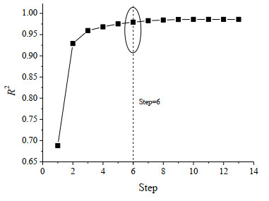
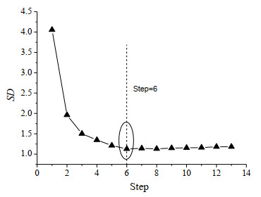
In the stepwise regression, the correlation coefficient (R2) and standard deviation (SD) changed with the introduction of variables. For the convenience of visual analysis, the changes are plotted in Figs. 1 and 2. It can be found from Fig. 1 that the correlation coefficient (R2) increased with the introduction of variables, and the initial increase trend was obvious. When the stepwise regression proceeded to step 6, the correlation coefficient (R2) approached the maximum, and then the correlation coefficient (R2) increase trend was slowing down. Similarly, it can be found in Fig. 2 that the standard deviation (SD) gradually decreased with the introduction of variables, and the initial decrease trend was obvious. When the stepwise regression proceeded to step 6, the standard deviation (SD) reached the minimum value, and then the standard deviation (SD) increased slightly.
Figure 1
 Figure 1. Changes of R in stepwise regression
Figure 2
 Figure 2. Changes of SD in stepwise regression
The regression diagnosis of the 6-variable model found that the variance inflation factor (VIF) of the variable x3 was the largest to be 6.835. No obvious colinearity was found between the variables. When the variables continued to be introduced, the stepwise regression proceeded to step 7. Although the correlation coefficient (R2) increased slightly, the variance inflation factor (VIF) of the variable x3 was 19.875, which was significantly greater than 10, indicating that the 7-variable model was unreliable. After considering all aspects, the combination of the variables obtained in step 6 of stepwise regression was chosen to build the model (M1), as shown in equation (6).
$ t_\text{R} = –1.4086 + 0.1445x_{2} – 0.4607x_{3} + 9.2865x_{5} – 0.8349x_{8} + 2.4593x_{9} + 0.7453x_{12 } (6) $ (6) $ N = 39, n = 9, m = 6, R^{2} = 0.9791, R_{CV}^{2} = 0.8542, SD = 1.1303, F = 249.1136; R_\text{test}^{2} = 0.9802, SD_\text{test} = 0.8333 $ N is the number of training set samples; n is that of test set samples; and m is that of variables. The correlation coefficient (R2) of the model (M1) is as high as 0.9791, which is far greater than the standard of 0.80; the standard deviation (SD) is 1.1303, and the chromatographic retention time range of the 39 training set samples is 32.68 – 3.07 = 29.61, SD/Vr = 1.1303/29.61 = 3.82%, which is far less than the standard of 10%, indicating that the model has a good fitting ability. The correlation coefficient (RCV2) of the cross test is 0.8542, which is much larger than the standard of 0.50, indicating this model has good stability. The correlation coefficient (Rtest2) of the test samples set, 0.9802, is much larger than the standard of 0.50; the standard deviation (SDtest) of the test set samples is 0.8333, and the chromatographic retention time range of the test set samples is 26.2 – 7.95 = 18.26, 0.8333/18.26 = 4.56%, which is far less than the standard of 10%, so the model has high prediction accuracy and strong prediction ability.
3.2.2 Partial least-squares regression model
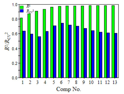
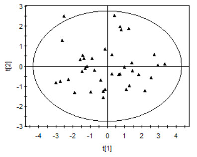
The partial least-squares regression (PLS) is also one of the commonly used methods in studying the relationship between the structure and properties of compounds, and is particularly suitable for modeling with a small number of samples and a large number of variables. The variables x1, x2, x3, ..., x13 of the samples (N = 39, n = 9) were used as independent variables X, and the compound chromatographic retention time (tR) as the dependent variable Y. A partial least-squares regression model (M2) was established. The change of the correlation coefficient (R2) and the correlation coefficient (RCV2) of the cross-test with the number of principal components (A) is shown in Fig. 3. It can be seen in this figure that when the number of principal components (A) reached 6, the correlation coefficient (R2) approached the maximum value, and the correlation coefficient (RCV2) of the cross test reached the maximum value. Six principal components should be selected for modeling (M2). The scatter distribution of the first two principal component scores of the 39 training set samples is plotted in Fig. 4. It can be found that the score points of most samples studied fell within the ellipse confidence circle with 95% confidence, and only one (less than 3%) outlier appeared. The above results reflect that the structure descriptors constructed can excellently represent the molecular structure characteristics of allergenic fragrance compounds, and get correct performance in statistical models.
Figure 3
 Figure 3. Correlation coefficient (R2/RCV2) change withthe number of principal components
Figure 4
 Figure 4. Distribution of the top 2 principal component scores of the sample
The correlation coefficient (R2) of the PLS model (M2) is 0.9744, which is much larger than the standard of 0.80; the standard deviation (SD) is 1.1461, SD/Vr = 1.1461/29.61 = 3.87%, which is much smaller than the standard of 10%, indicating that the model has good fitting ability. The correlation coefficient (RCV2) of the cross test, 0.7464, is much larger than the standard of 0.50, indicating good stability for the model. The correlation coefficient (Rtest2) of the test set samples is 0.9367, which is much larger than the standard of 0.50; the standard deviation of the test set samples (SDtest) is 0.8333, and the range of the chromatographic retention time of the test set samples is 26.2 – 7.95 = 18.26, 1.4903/18.26 = 8.16%, which is far less than the 10% standard, and thus the model has high prediction accuracy and strong prediction ability.
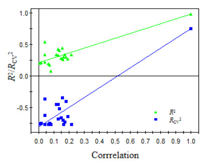
The R2 and RCV2 of the models are plotted in Fig. 5 with the correlation coefficients of the Y original vector and the randomly ordered Y vector. According to the judgment standard proposed by Andersson et al.[29], the intercepts of R2 and RCV2 on the vertical axis must not exceed 0.300 and 0.050, respectively. It can be seen from Fig. 5 that the intercepts of R2 and RCV2 of the PLS model constructed in this paper are 0.211 and –0.805, respectively, both below the critical value, which fully demonstrates that the excellent results of the above model were not caused by accidental factors. The partial least-squares regression model (M2) can be used to analyze the influence of compound structural factors on the chromatographic retention time.
Figure 5
 Figure 5. Y vector random sorting verification
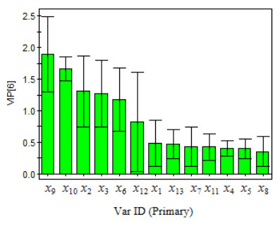
The importance of a variable can reflect the degree of correlation between independent variables X and Y. It is generally believed that a variable with an importance projection (VIP) value greater than 1 has a large correlation with the chromatographic retention time (tR) of the compound. The importance projection of the variables is shown in Fig. 6, which shows that the VIP values of the five variables x9, x10, x2, x3 and x6 are greater than 1, indicating that these five variables are highly correlated with the compound's chromatographic retention time (tR). The top three x9, x10 and x2 are all related to the 2nd type of non-hydrogen atoms, and the number of the 2nd type of non-hydrogen atoms determine the chain length, reflecting that the greater the number of the 2nd type of non-hydrogen atoms in a compound, the larger value of chromatographic retention time (tR) for the compound, which is basically consistent with the characteristics of the Table 1 data.
Figure 6
 Figure 6. Projection of variable importance
3.2.3 Model results and comparison
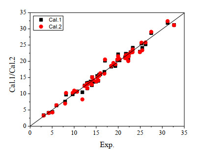
The multiple linear regression (MLR) model (M1) and partial least-squares regression (PLS) model (M2) calculated the chromatographic retention time of the compounds in the training set, and predicted the chromatographic retention time of the compounds in the test set that were not involved in the modeling. The calculated and predicted values of M1 and M2 for the compounds are listed in the Cal.1 and Cal.2 columns of Table 1, respectively. The correlation between the calculated values of the retention times and the experimental values of the two models is shown in Fig. 6. It is easy to see in Fig. 6 that all the sample points fall near the 45° diagonal of the square, indicating that the calculated values of the compound retention time in the two models are well correlated with the experimental values, and the errors are not large. In addition, it can be seen from the figure that the distribution of the sample points of Cal.1 and Cal.2 are generally similar, indicating that the quality of models M1 and M2 is roughly equivalent.
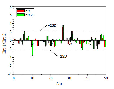
The errors of the model's calculation of compounds' retention time can reflect the accuracy of the model's prediction. The calculation error distribution of the two models is shown in Fig. 8, in which the prediction error values of most of the samples are within the range of 2 times of standard deviations (±2SD), and only 2 compounds (6.25%) are outside this range, which indicates that these two models are accurate in predicting the retention time of the compounds. The resulting errors are small and all within acceptable limits. In addition, err.1 of most samples are smaller than err.2, so model M1 has slightly more excellent quality than M2. The samples studied in this paper have a large structure span, including olefins, alcohols, ethers, phenols, esters and other types of compounds, containing heteroatoms such as oxygen and nitrogen, and containing single, double, and triple bonds, as well as cyclic, and benzene rings. The results obtained in this paper are very satisfactory for a sample system with complex composition and large structure span.
Figure 7
 Figure 7. Correlation diagram between the model predicted and experimental values
Figure 8
 Figure 8. Model prediction errors of samples' tR
There have been some reports[30-32] on the relationship between quantitative structure and retention time of complex sample systems. For comparison, the results of this article and some literatures are listed in Table 3. It can be found in Table 3 that the results obtained in this paper are better than the reports.
Table 3
Table 3. Comparisons among Different QSRR ModelsDownLoad:
CSV
No. Descriptor N m/A Method R2 R Rtest2 SD Vr SD/Vr F 1[30] MEDVR 55 8 MLR 0.978 0.989 — 1.366 34.28 3.98% — 2[30] MEDVR 55 4 PLS 0.974 0.987 — 1.397 34.28 4.08% — 3[31] I-MEDV 37 9 MLR 0.960 0.980 — 0.991 23.34 4.25% 74.389 4[31] I-MEDV 37 4 MLR 0.951 0.975 — 1.032 23.34 4.42% 152.688 5[32] MEDV 46 10 MLR 0.821 0.906 — — 38.339 — — 6[32] MEDV 46 6 MLR 0.815 0.903 — — 38.339 — — 7* MVVR 39 6 MLR 0.9791 0.9894 0.9802 1.1303 29.61 3.82% 249.1136 8* MVVR 39 6 PLS 0.9744 0.9871 0.9367 1.1461 29.61 3.87% — "—": not available; "*": results of this work 4. CONCLUSION
New structure descriptors were obtained by constructing relationship between non-hydrogen atoms. The structures of 48 common allergenic fragrance organic compounds were parameterized. The multiple linear regression (MLR) and partial least-squares regression (PLS) were used to build models of the relationship between compound structure and chromatographic retention time. After testing, the models have good fitting ability, stability and external prediction ability. The structural factors affecting the chromatographic retention time of the compounds were analyzed. The results show that the compound with more secondary carbon atoms likely shows larger chromatographic retention time (tR) value. The compound structure descriptors constructed are two-dimensional structure descriptors, which are simple, fast, easy to understand, and highly versatile. This research has certain reference value for studying the relationship between the structures and properties of compounds.
-
-
[1]
Cheng, Y.; Wang, C.; Xue, Y. M.; Chen, W.; Wang, X.; Bai, H.; Cai, T. P.; Hu, K. X. Determination of dicumarol and cyclocoumarol in cosmetics by HPLC/DAD. J. Anal. Test. 2008, 27, 1996–1999.
-
[2]
Xi, H. W.; Ma, Q.; Liu, Q.; Wang, Y.; Ding, L; Su, N.; Bai, H.; Wang, C. HPLC-MS/MS determination of nonylphenol in cosmetics. J. Instrumental Anal. 2010, 29, 46–50.
-
[3]
Jiang, J. H.; Chen, S.; Xie, J. X. Analysis of ten harmful fragrances in cosmetics by GC/FTIR. Chin. J. Health Lab. Technol. 2005, 15, 1415–1418.
-
[4]
Li, Z. Y.; Wei, S. W.; Zhu, Z. J.; Jin, J. L. Determination of odorous substances in textile by solvent extraction GC-MS. Chem. Anal. Meterage 2011, 20, 35–37.
-
[5]
Gu, J. H.; Pan, K.; Liu, Y.; Zhu, Z. H. Determination of eugenol in fragrant fabrics by GC/MS method. Chin. Dyeing Finishing 2014, 40, 40–45.
-
[6]
Gao, M. X.; Wang, X. Y.; Gong, Y.; Wang, H.; Liao, Q. Detection of nonanal aromatic in coated fabrics by headspace gas chromatography-mass spectrometry. Anal. Instr. 2011, 42, 32–35.
-
[7]
Wu, X. H.; Zhu, R. Z.; Lu, S. M.; Wang, K.; Meng Z. J.; Mou, D. R.; Miao, M. M. UHPLC-MS/MS determination of coumarin in essence. Phys. Test Chem. Anal. Part B: Chem. Anal. 2000, 5, 1407–1400.
-
[8]
Wei, B. W.; Dai, X. W.; Yang, L.; Yang, R. J. Determination of fragrance allergens in toys by gas chromatography-ion trap mass spectrometry. Enciron. Chem. 2013, 32, 2406–2410.
-
[9]
Chen, L. Q.; Lin, Z. H.; Xing, Y. N.; Feng, A. H.; Wang, X.; Chen, Z. Y. Determination of fragrance allergens in toys by gas chromatography-mass spectrometry. Chin. J. Anal. Lab. 2014, 33, 1171–1176.
-
[10]
Li, H. Y.; Bai, H.; Lv, Q.; Li, P.; Wang, X.; Guo, X. Y.; Zhang, Q. A method for fast screening of allergenic fragrance substance in plushtoys. Chin. J. Anal. Chem. 2013, 41, 1518–1525.
-
[11]
Baviskar, B. A.; Deore, S. L.; Alone, S. 2D QSAR study on saponins of pulsatilla koreana as an anticancer agent. Pharm. Commun. 2019, 9, 2–6.
-
[12]
Abdel-Aziz, H. A.; Eldehna, W. M.; Fares, M.; Al-Rashood, S. T. A.; Al-Rashood, K. A.; Abdel-Aziz, M. M.; Soliman, D. H. Synthesis, biological evaluation and 2D-QSAR study of halophenyl bis-hydrazones as antimicrobial and, antitubercular agents. Int. J. Mol. Sci. 2015, 16, 8719–8743. doi: 10.3390/ijms16048719
-
[13]
Khan, K.; Khan, P. M.; Lavado, G.; Valsecchi, C.; Pasqualini, J.; Baderna, D.; Marzo, M.; Lombardo, A.; Roy, K.; Benfenati, E. QSAR modeling of daphnia magna and fish toxicities of biocides using 2D descriptors. Chemosphere 2019, 229, 8–17. doi: 10.1016/j.chemosphere.2019.04.204
-
[14]
Yu, W.; He, H. M.; Feng, C. J. QSAR models for the inhibitory enzyme activities of triazinyl-oxadiazolyl-pyrazole derivatives. Chemistry 2018, 81, 636–640. doi: 10.7524/j.issn.0254-6108.2017102301
-
[15]
Cai, W. P.; Wei, X. C.; Zheng, C.; He, L.; Zhao, W. Z.; Zheng, X. A 3D-QSAR model of the tyrosinase inhibitory activity of curcumin analogues. Mod. Food Sci. Technol. 2017, 33, 41–50.
-
[16]
Kaur, M.; Silakari, O. Ligand-based and e-pharmacophore modeling, 3D-QSAR and hierarchical virtual screening to identify dual inhibitors of spleen tyrosine kinase (Syk) and janus kinase 3 (JAK3). J. Biomol. Struct. Dyn. 2017, 35, 1–18. doi: 10.1080/07391102.2015.1136896
-
[17]
Chen, Y. Z.; Fan, X. J.; Zhang, H.; Liang, G. Z.; Liu, B. G. 3D-QSAR and interaction mechanism of flavonoids as aldose reductase inhibitors based on topomer Comfa and surflex-dock. J. Henan Univ. Technol. (Nat. Sci. Ed. ) 2018, 39, 91–96.
-
[18]
Misra, S.; Singh, H.; Kim, K.; Perez-Sanchez, H. S.; Kim, M.; Kumar, S.; Yadav, D. K.; Jang, C.; Choi, E. H.; Mancera, R. L.; Sharma, P. Studies of the benzopyran class of selective COX-2 inhibitors using 3D-QSAR and molecular docking. Arch. Pharmacal Res. 2018, 41, 1178–1189 doi: 10.1007/s12272-017-0945-7
-
[19]
Cui, S. H.; Niu, Z. Y.; Zhang, X. M.; Qin, L. Y.; Luo, X. Determination of 48 fragrance allergens in plastic toys by gas chromatography-mass spectrometry. J. Chin. Mass Spectrom. Soc. 2016, 37, 163–172.
-
[20]
Li, J. F.; Xie, Y. H.; Lei, Y. H. Study on relationship of structure and change in heat capacity for some polymers. Compu. Appl. Chem. 2016, 33, 833–837. http://en.cnki.com.cn/Article_en/CJFDTOTAL-JSYH201607018.htm
-
[21]
Li, J. F. Study on acute toxicity for halogenated phenols by using molecular vertex electronegativity interaction vector. Comput. Appl. Chem. 2015, 32, 1399–1403.
-
[22]
Liao, L. M. Research on structure-retention index relationship of aldehydes and ketones. Chem. Res. Appl. 2015, 27, 617–623.
-
[23]
Liao, L. M.; Huang, X.; Lei, G. D. Structural characterization and octanol/water partition coefficient (LogP) prediction for oxygen-containing organic compounds. Chin. J. Struct. Chem. 2017, 36, 1243–1250.
-
[24]
Qin, Z. L. A new connectivity index for QSPR/QSAR study of alcohol. J. Xuzhou Normal Univ. (Nat. Sci Ed. ) 2001, 19, 50–52.
-
[25]
Du, X. H. Predicting the lgKow of PCDDs using novel topological parameter. J. Wuhan Univ. Technol. 2007, 29, 40–44. http://www.en.cnki.com.cn/Article_en/CJFDTotal-WHGY200701010.htm
-
[26]
Chen, Y. Prediction of aqueous solubility, hydrophobic parameter for esters and ketones with novel valence connectivity index. J. Nanjing Univ. Technol. 2005, 27, 41–43.
-
[27]
Xu, Qi; Fan, L. L.; Xu, J. A simple 2D-QSPR model for the prediction of setschenow constants of organic compounds. Maced. J. Chem. Chem. Eng. 2016, 35, 53–62.
-
[28]
Gramatica, P.; Pilutti, P.; Papa, E. A tool for the assessment of VOC degradability by tropospheric oxidants starting from chemical structure. J. Chem. Inf. Comput. Sci. 2004, 44, 1794–1802.
-
[29]
Andersson, P. M.; Sjstrom, M.; Lundstedt, T. Preprocessing peptides sequences for multivariate sequence-property analysis. Chemom. Intell. Lab. Syst. 1998, 42, 41–50.
-
[30]
Liao, L. M.; Li, J. F.; Qing, D. H.; Lei, G. D. Structural characterization and retention time prediction for components of essential oil of meconopsis integrifolia flowers. Chin. J. Struct. Chem. 2010, 29, 1638–1645.
-
[31]
Liao, L. M.; Zhu, J.; Li, J. F.; Lei, G. D. QSRR study on components of styrax japonicus sieb flowers using improved molecular electronegativity-distance vector (I-MEDV). Chin. J. Struct. Chem. 2011, 30, 105–110.
-
[32]
Zhu, W. P.; Mei, H.; Shu, M.; Liao, L. M.; Yang, J.; Li, Z. L. Structural characterization of some components from essential oils of rosa banksiae ait for estimation and prediction of their linear retention index and retention times. Chin. J. Chin. Mater. Med. 2008, 33, 609–611.
-
[1]
-
Figure 3 Correlation coefficient (R2/RCV2) change withthe number of principal components
Table 1. 48 Allergenic Fragrances and Their Chromatographic Retention Time
No. Compounds tR(Exp.) Cal.1 Cal.2 1 Ethyl acrylat 3.07 3.37 3.27 2 Ethyl trans-2-butenoate 4.21 4.11 4.08 3 5-Methyl-2, 3-hexanedione 5.06 4.38 4.24 4 Trans-2-hexenal diethyl acetal 5.98 6.39 6.45 5* Trans-2-heptenal 7.95 7.57 6.97 6 d-Limonene 8.16 9.74 10.23 7 Trans-2-hexenal dimethyl acetal 9.67 9.84 10.29 8 Linalool 10.02 10.58 10.96 9 Benzyl alcohol 10.65 10.74 10.60 10* Dimethyl citraconate 11.87 10.47 8.25 11 Citronellol 12.38 12.51 12.42 12 Methyl heptine carbonate 12.90 13.28 13.01 13 Diethyl maleate 12.98 11.66 11.69 14 Geraniol 13.07 13.12 12.97 15* Benzyl cyanide 13.23 13.39 13.05 16 Citral 13.73 13.77 13.44 17 4-Methoxyphenol 14.02 12.64 12.84 18 Hydroxy-citronellal 14.08 15.11 15.10 19 4-Tert butylphenol 14.36 13.69 14.25 20* 4-Ethoxy-phenol 14.99 13.75 13.79 21 Cinnamaldehyde 15.24 15.49 14.97 22 Anisyl alcohol 15.47 13.99 14.14 23 Cinnamylalcohol 15.70 15.89 15.53 24 Eugenol 15.95 16.04 16.31 25* Trans-4-phenyl-3-butene-2-one 16.87 16.73 16.20 26 3-Methyl-4-(2, 6, 6-trimethyl-2-cyclohexen-1-yl)-3-buten-2-one 17.00 20.2 20.57 27 Isoeugenol 18.42 18.36 18.59 28 Dihydro coumarin 18.90 18.92 19.47 29 2-(4-Tert-butylbenzyl)propionaldehyde 19.35 18.56 19.08 30* 2, 4-Dihydroxy-3-methylbenzaldehyde 19.80 20.38 20.57 31 6, 10-Dimethyl-3, 5, 9-undecatrien-2-one 19.99 22.16 21.57 32 Coumarin 20.31 20.29 20.66 33 Amylcinnamyl alcohol 21.56 21.19 20.99 34 Amyl cinnamal 21.74 22.32 21.90 35* Farnesol 21.83 21.04 20.92 36 6-Methylcoumarin 22.29 20.62 20.07 37 7-Methylcoumarin 22.34 21.71 22.08 38 Hydroxyisohexyl 22.38 22.23 21.47 39 Diphenylamine 22.83 22.8 22.71 40* Hexyl cinnamaldehyde 23.25 23.32 22.8 41 4-(4-Methoxyphenyl)-3-butene-2-one 23.32 24.16 23.68 42 1-(4-Methoxyphenyl)-1-penten-3-one 24.92 22.95 22.83 43 Benzyl benzoate 25.29 25.5 25.74 44 Musk ambrette (4-tert-butyl-3-methoxy-
2, 6-dinitrotoluene)25.46 24.14 23.41 45* 7-Methoxycoumarin 26.21 25.26 25.81 46 Benzyl salicylate 27.50 28.72 29.09 47 7-Ethoxy-4-methylcoumarin 31.22 31.82 32.38 48 Benzyl cinnamate 32.68 31.19 31.12  下载: 导出CSV
Table 2. Structurally Parameterized Characterization Results of the Compounds
No. x1 x2 x3 x4 x5 x6 x7 x8 x9 x10 x11 x12 x13 1 3.9568 2.9954 1.8708 0.0000 0.0635 2.8006 2.7979 0.0000 1.8765 2.3820 0.0000 0.0000 0.0000 2 3.7321 4.5765 1.8708 0.0000 0.0043 2.8296 2.4296 0.0000 2.3075 2.8966 0.0000 0.0000 0.0000 3 6.4641 1.4142 5.4737 0.0000 0.6531 0.9528 9.8244 0.0000 0.0000 3.4973 0.0000 2.7426 0.0000 4 3.0000 8.8191 1.7321 0.0000 0.0000 2.7851 0.0585 0.0000 2.9767 3.0520 0.0000 0.0000 0.0000 5* 2.7321 8.9861 0.0000 0.0000 0.0000 3.7647 0.0000 0.0000 3.7215 0.0000 0.0000 0.0000 0.0000 6 3.2247 5.8238 5.4737 0.0000 0.2131 0.5961 4.4432 0.0000 3.8009 8.9009 0.0000 2.0200 0.0000 7 4.4142 5.9907 0.0000 2.0000 0.2663 1.7305 0.0000 3.4074 4.3718 0.0000 2.5159 0.0000 0.0000 8 5.6390 5.9907 1.8708 2.0000 0.4100 3.0629 2.2695 3.4771 4.5041 2.5293 4.0515 0.0000 0.0021 9 1.4142 9.3199 1.8708 0.0000 0.0000 1.3851 0.4120 0.0000 4.7423 6.7777 0.0000 0.0000 0.0000 10* 6.4641 1.5811 5.6125 0.0000 0.1487 0.9719 7.7275 0.0000 0.0000 4.3355 0.0000 2.9378 0.0000 11 4.4142 7.2380 3.6029 0.0000 0.1360 2.6244 3.3536 0.0000 5.3963 6.1941 0.0000 0.0018 0.0000 12 3.7321 9.1210 1.8708 0.0000 0.0518 2.0236 2.7011 0.0000 5.5929 3.1334 0.0000 0.0000 0.0000 13 5.4641 5.9907 3.7417 0.0000 0.0046 3.2549 4.8085 0.0000 5.6232 5.7934 0.0000 0.0684 0.0000 14 4.4142 7.4049 3.7417 0.0000 0.1364 2.7528 3.4569 0.0000 5.6572 7.0112 0.0000 0.0020 0.0000 15* 1.4142 11.0520 1.8708 0.0000 0.0000 2.2242 0.0556 0.0000 5.7177 7.2163 0.0000 0.0000 0.0000 16 4.7321 7.5718 3.7417 0.0000 0.1375 3.6945 3.4978 0.0000 5.9067 6.9500 0.0000 0.0020 0.0000 17 2.4142 6.3246 3.7417 0.0000 0.0000 1.0171 2.0562 0.0000 6.0164 10.1946 0.0000 0.0896 0.0000 18 5.8284 5.9907 5.3349 0.0000 0.2052 2.8350 6.0687 0.0000 6.0391 6.7682 0.0000 1.8214 0.0000 19 4.4142 6.3246 3.7417 2.0000 0.4060 1.0904 2.4823 3.6392 6.1449 10.1946 1.1590 0.0896 2.2733 20* 2.4142 7.7388 3.7417 0.0000 0.0000 1.8036 1.7542 0.0000 6.3831 10.6662 0.0000 0.0896 0.0000 21 1.7321 12.6491 1.8708 0.0000 0.0000 2.6965 0.0050 0.0000 6.4776 7.6559 0.0000 0.0000 0.0000 22 2.4142 6.3246 3.7417 0.0000 0.0000 1.0171 2.0562 0.0000 6.5646 10.1946 0.0000 0.0896 0.0000 23 1.4142 12.4822 1.8708 0.0000 0.0000 1.6848 0.0019 0.0000 6.6515 7.6411 0.0000 0.0000 0.0000 24 3.6390 7.7388 5.6125 0.0000 0.0016 2.1928 2.6321 0.0000 6.7461 12.3320 0.0000 3.1052 0.0000 25* 2.7321 11.0680 3.7417 0.0000 0.3476 0.9643 3.5087 0.0000 7.0939 10.0294 0.0000 0.0684 0.0000 26 6.7321 5.9907 7.3445 2.0000 0.5391 1.1156 7.8522 2.4493 7.1430 7.8670 2.5777 4.8259 2.6599 27 3.4142 7.9057 5.6125 0.0000 0.0016 1.7668 2.6252 0.0000 7.6799 12.7720 0.0000 3.1052 0.0000 28 1.4142 9.1530 5.6125 0.0000 0.0000 0.4462 2.0171 0.0000 7.8614 10.8853 0.0000 3.0307 0.0000 29 5.4142 9.3199 5.4737 2.0000 0.4347 2.2288 2.3246 3.6392 8.0315 15.0667 1.1591 0.5282 2.2733 30* 5.5605 4.7434 7.4833 0.0000 0.0583 2.7033 7.6738 0.0000 8.2016 8.9393 0.0000 8.4499 0.0000 31 5.7321 9.1530 5.6125 0.0000 0.4829 2.0449 6.9067 0.0000 8.2735 9.4907 0.0000 0.0052 0.0000 32 1.7321 9.4868 5.6125 0.0000 0.0000 0.6260 2.2610 0.0000 8.3945 12.2359 0.0000 3.0426 0.0000 33 2.4142 16.7248 3.6029 0.0000 0.0000 1.7904 1.5935 0.0000 8.8671 11.5315 0.0000 0.0527 0.0000 34 1.0000 18.1390 1.8708 0.0000 0.0000 1.0653 0.0000 0.0000 8.9351 7.6426 0.0000 0.0000 0.0000 35* 5.4142 11.8145 5.6125 0.0000 0.1364 3.2594 4.5916 0.0000 8.9691 11.5362 0.0000 0.0039 0.0000 36 2.7321 9.4868 3.7417 2.1213 0.0000 1.1813 3.3163 0.1260 9.1431 7.3566 8.0977 0.0043 1.4857 37 2.7321 7.9057 7.4833 0.0000 0.0000 1.6525 3.4456 0.0000 9.1620 17.4514 0.0000 3.8813 0.0000 38 3.4142 4.2426 1.7321 0.0000 0.1354 2.0536 2.1022 0.0000 9.1771 1.8444 0.0000 0.0000 0.0000 39 0.0000 17.4847 3.7417 0.0000 0.0000 0.0000 0.0000 0.0000 9.3472 14.5556 0.0000 0.5659 0.0000 40* 2.7321 18.1390 3.7417 0.0000 0.0000 3.2075 0.7340 0.0000 9.5060 13.1333 0.0000 0.6089 0.0000 41 3.7321 9.4868 5.6125 0.0000 0.3476 1.0384 3.8422 0.0000 9.5325 15.0549 0.0000 0.1580 0.0000 42 3.7321 10.9010 5.6125 0.0000 0.0351 2.1410 2.9594 0.0000 10.1374 16.6615 0.0000 0.1580 0.0000 43 1.7321 17.2256 5.6125 0.0000 0.0000 0.2568 3.1008 0.0000 10.2773 13.7172 0.0000 2.3221 0.0000 44 11.9282 1.5811 13.7813 2.0000 2.1253 0.2673 17.7876 3.6414 0.0000 5.8014 0.5176 20.0867 3.0398 45* 2.7321 7.9057 7.4833 0.0000 0.0000 0.6980 2.5969 0.0000 10.6251 16.0981 0.0000 3.8229 0.0000 46 3.1463 15.6445 7.4833 0.0000 0.0044 0.6984 5.4745 0.0000 11.1128 14.4093 0.0000 5.2982 0.0000 47 3.7321 7.7388 9.3541 0.0000 0.0019 1.7069 3.8928 0.0000 12.5193 16.1399 0.0000 7.5301 0.0000 48 1.7321 20.3879 5.6125 0.0000 0.0000 0.7689 2.3768 0.0000 13.0713 17.2862 0.0000 0.1275 0.0000
下载: 导出CSV
Table 3. Comparisons among Different QSRR Models
No. Descriptor N m/A Method R2 R Rtest2 SD Vr SD/Vr F 1[30] MEDVR 55 8 MLR 0.978 0.989 — 1.366 34.28 3.98% — 2[30] MEDVR 55 4 PLS 0.974 0.987 — 1.397 34.28 4.08% — 3[31] I-MEDV 37 9 MLR 0.960 0.980 — 0.991 23.34 4.25% 74.389 4[31] I-MEDV 37 4 MLR 0.951 0.975 — 1.032 23.34 4.42% 152.688 5[32] MEDV 46 10 MLR 0.821 0.906 — — 38.339 — — 6[32] MEDV 46 6 MLR 0.815 0.903 — — 38.339 — — 7* MVVR 39 6 MLR 0.9791 0.9894 0.9802 1.1303 29.61 3.82% 249.1136 8* MVVR 39 6 PLS 0.9744 0.9871 0.9367 1.1461 29.61 3.87% — "—": not available; "*": results of this work
下载: 导出CSV
-


 扫一扫看文章
计量
- PDF下载量: 1
- 文章访问数: 591
- HTML全文浏览量: 9
 下载:
下载:
